Numerical study of the antiferromagnetic Ising model on a hypersphere

Abstract

We built a model where all spins are in interaction with each other via an antiferromagnetic Ising Hamiltonian. The geometry of such a model is a tetrahedron placed on a hypersphere in spaces of dimensions enclosed between 1 and 9. Due to confinement and to the fact that all spins interact which each other, our spin system exhibit frustration. The temperatures of the observed antiferro-paramagnetic transitions are equal for all space dimensions to one of two given values depending on the parity of the space dimension. Moreover, the order parameter $<m>$, i.e. the magnetization of the system, has been also studied.

The Ising model has been widely studied to understand physical phenomena that occur in ferro or antiferroelectric compounds, lattice gas, binary alloys etc. But, up to now, there are very few articles on confinement effects binder ; diehl ; dosch ; drze on the Ising model. Understanding the statistical mechanics of classical systems in confined geometries and in systems of small sizes is important for the future studies of nanocompounds.

This article deals of $N$ Ising spins on a $d=N-2$ dimensional hypersphere. The geometry of the spins corresponds to the following: each spin is located on the apex of the tetrahedron corresponding to the space dimension. For the sake of confinement, we assume that the space is closed: it corresponds to a $d$ dimensional hypersphere on which the tetrahedron is located. This tetrahedron is located on the hypersphere so as each spin is at equal distance from each other. Hence the curvature of the hypersphere is very large and is directly related to the distance between spins. The number of apex of the tetrahedron is also directly related to the dimension of space: if $d$ is the dimension of hyperspace, the number of apex is equal to $d+2$. So, like in a 1-dimensional circle or a 2-dimensional sphere, each spin located at an apex of the tetrahedron is at equal distance from all other spins.

Hence the Hamiltonian of such an Ising model writes:

$$H=-\sum_{i}\sum_{j\neq i}-Js_{i}s_{j}$$ (1)

were $s_{i}$ is Ising spin number $i$ and $J<0$ is the antiferromagnetic coupling. We took here the magnetisation $m=<|s_{i}|>$ of the assembly of spins as the order parameter in a finite size analysis. The algorithm used here was the Wolff one.

The finite size analysis 40 is a very efficient way to study phase transitions by Monte-Carlo simulations. Indeed, the notion of phase transi tion has a sense only for the thermodynamical limit, while simulations can only be done on finite size systems. For the case of second order phase transitions, for infinite size systems with periodic boundary conditions, the correlation length diverges at the critical temperature $T_{c}$. Here, we have a closed and finite space.

We shall define here the physical parameters necessary to the finite size analysis. The specific heat per spin $c$ writes:

$$c(t)=\frac{<E^{2}>-<E>^{2}}{Nk_{B}T^{2}}$$ (2)

where $E$ is the total energy of the assembly of spins, $T$ is the the absolute temperature, $k_{B}$ is Boltzmann constant and $t=T/T_{c}-1$ where $T_{c}$ is the critical temperature. For the order parameter per spin $m$ we have:

$$m(t)=\frac{<|M|>}{N}$$ (3)

where $M$ is the magnetization of the whole assembly of spins. We took $J=1$ and $k_{B}=1$. The results are the following.

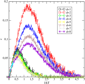
Figure 1: Evolution of the specific heat $c$ as a function of $\beta=1/k_{B}T$ for space dimensions : $d=1,2,3,4,5,6,7,8,9$

In fig.1, one can see the evolution of the specific heat $c$ as a function of $\beta$. For low space dimensions $d<10$ it appears a smooth maximum in this graph which can be interpreted as a transition at a critical temperature $\beta_{c}$. It is easy to see that if the curved space has a dimension which is odd the inverse of the critical temperature is equal to $\beta_{c}=0.6$; if the hypersphere has an even space dimension the critical temperature is equal to $\beta_{c}=1.25$. This is valid for all space dimensions enclosed between $d=1$ and $d=9$. But for high dimensions, the evolution of the peak of $c$ seems to flatten as a function of $\beta$. Though, we have checked that transitions always occur for $N\rightarrow\infty$ and that the two values of $\beta_{c}$ remain. Let us look now at fig.2 which is the evolution of the order parameter $<m>$ as a function of the inverse temperature $\beta=1/k_{B}T$. For $d=2$ and $d=4$, $<m>$ tends to zero when $\beta$ tends to infinity. For the space dimension $d=1,3,5,6,7,8,9$ even for $\beta\rightarrow\infty$ the magnetization $<m>$ does not tend to zero.

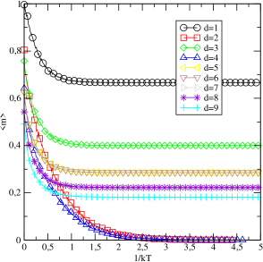
Figure 2: Evolution of the order parameter $<m>$ as a function of $\beta=1/k_{B}T$ for space dimensions : $d=1,2,3,4,5,6,7,8,9$

To resume fig.2 we plotted in fig. 3 the values of $<m>$ at $\beta=0$ (squares) and at $\beta=5$ (circles). For $d=100$ we add the value of $<m>=0.156$ at $\beta=0$ and $<m>=0$ at $\beta=5$.

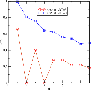
Figure 3: Evolution of the $<m>$ at $1/k_{B}T=5$ (circles) and at $1/k_{B}T=0$ (squares) as a function of space dimension $d$

Geometrical frustration mosseri is the explanation of the behavior of both $<m>$ and $c$ as a function of $\beta$. $<m>$ at $1/k_{B}T=5$ is equal to zero for $d=2$ and for $d=4$ because the number of antiferromagnetic spins is even in such spaces and geometrical frustration is not too strong. Hence it is possible that the number of spins up and the number of spins down is equal even if geometrical frustration remains because of the tetrahedral geometry. For even space dimensions larger than 4, geometrical frustration is too strong, and the number of spins up and down is different leading to a non zero value of the magnetization as the temperature goes to zero (i.e. $\beta\rightarrow\infty$).

If the space dimension is even, the number of spins is also even, hence the transition from an antiferromagnetic state to a paramagnetic one will occur at a lower temperature, i.e. at a larger $\beta$ value because each spin has $d+1$ neighbours. Hence, the number of interactions between spins is odd and $<E>^{2}$ always differs from $<E^{2}>$ of one value of spin interaction. For odd space dimensions, the even number of interactions between spins renders it possible that $<E^{2}>$ is close to $<E>^{2}$, transitions occur at a larger temperature (i.e. lower $\beta$).

The values of the critical temperature are the same for all odd (resp. even) space dimensions: the tetrahedral geometry is the same in all dimensions, no critical dimension has been observed because of the curvature of space. Moreover, we don not observe, as the number of spins increases, that the critical value $\beta_{c}$ tends to zero, contrarily to large systems in a threedimensional space.

This work has been done with the financial support of a CNRS-FONACIT contract.

References

- (1) K.Binder, in Phase Transitions and Critical Phenomena, edited by C.Domb and J.L.Lebowitz (Academic, London, 1983), Vol. 8, p.1
- (2) H.Diehl, in Phase Transitions and Critical Phenomena, edited by C.Domb and J.L.Lebowitz (Academic, London, 1983), Vol.10, p.75
- (3) H.Dosch, in Critical Phenomena at Surfaces and Interfaces edited by G.Höhler and E.A. Niekish (Springer, Berlin, 1992), Vol. 126, p. 1
- (4) A.Drzewinski, Phys. Rev. E 62 (2000) 4378
- (5) M.E.Fisher and M.N.Barber, Phys. Rev. Lett. 28 (1972) 1516
- (6) G.S.Rushbrooke, J.Chem. Phys. 39 (1963) 842
- (7) J.F.Sadoc, R.Mosseri Frustration Géométrique (Editions Eyrolles, Paris 1997)