Abstract

The paper describes the SPHINX facility which includes a wide-aperture magnetic spectrometer with scintillation counters and hodoscopes, proportional chambers and drift tubes, multichannel electromagnetic and hadron calorimeters, a guard system, a RICH velocity spectrometer and a hodoscopical threshold Cherenkov detector for the identification of charged secondary particles. The SPHINX spectrometer, in its last modification, had the possibility to record $\sim 3000$–$4000$ trigger events per an accelerator burst. The spectrometer was used during the last decade in experiments with the 70 GeV proton beam of the IHEP accelerator U-70.

1 Introduction

In 1989–1999 extensive studies of diffractive-like baryon production and OZI suppressed reactions, searches for exotic and cryptoexotic pentaquark states and several other rare processes were carried out in experiments with the SPHINX facility at the proton beam of the IHEP accelerator with energy $E_{p}=70$ GeV. The SPHINX facility was the multipurpose wide-aperture spectrometer with the possibility of complete reconstruction of charged and neutral secondary particles. Over the time several modifications of the SPHINX detector were made and all the measurements can be divided into two stages:

• First generation experiments with the “old” setup, performed in 1989–1994. The main results of these measurements were published between 1994-2000 (see [1, 2, 3, 4, 5, 6, 7, 8, 9, 10, 11, 12, 13] and review papers [14, 15]). The short description of the first version of the SPHINX detector can be found in [1].

• Second generation experiments with the completely upgraded SPHINX detector, which is described in this paper.

The “old” and upgraded SPHINX setup had the same general structure. However, after the upgrade the facility was equipped with a new tracking system, new hodoscopes, a hadron calorimeter and a modernized RICH velocity spectrometer, new electronics, a new DAQ system and on-line computers. As a result we obtained, practically, a new setup which was capable to record an order of magnitude more data per spill.

The layout of the upgraded SPHINX detector is presented in Fig. 1. The right-handed $X,Y,Z$ coordinate system of the setup had $Z$-axis in the direction of the proton beam, vertical $Y$-axis and horizontal $X$-axis. The origin of the coordinate system was in the center of the Magnet.

Figure 1: Layout of the SPHINX spectrometer (plan view): $\mathrm{S}_{1}$–$\mathrm{S}_{4}$ — beam scintillation counters (the very upstream counters $\mathrm{S}_{1}$ and $\mathrm{S}_{2}$ are not shown in this figure); $\mathrm{T}_{1}$, $\mathrm{T}_{2}$ — copper and carbon targets; $\mathrm{A}_{1}$–$\mathrm{A}_{8}$ — lead-scintillator veto counters; $\mathrm{B}_{1}$–$\mathrm{B}_{2}$ — veto counters to tag non-interacting primary beam particles; $\mathrm{H}_{1X,Y}$, $\mathrm{H}_{2X,Y}$ — beam hodoscopes; $\mathrm{H}_{3}$ — side hodoscope around the target; $\mathrm{H}_{4X}$, $\mathrm{H}_{5X}$, $\mathrm{H}_{6X}$, $\mathrm{H}_{7}$, $\mathrm{H}_{8Y}$ — trigger hodoscopes; PC — proportional chambers; DT — drift tubes; RICH — velocity spectrometer with registration of the rings of Cherenkov radiation; Č — multichannel threshold Cherenkov counter; ECAL — electromagnetic calorimeter; HCAL — hadron calorimeter.

The main elements of the detector were as follows:

• The detectors of the primary proton beam — the scintillation counters $S_{1}-S_{4}$, $B_{1},B_{2}$ and the scintillator hodoscopes $H_{1X,Y},H_{2X,Y}$.

• The targets $T_{1}$, $T_{2}$ and the guard system — the hodoscope $H_{3}$ and the lead-scintillator veto counters $A_{1}-A_{8}$.

• The wide-aperture magnetic spectrometer consisted of the magnet, the block of proportional chambers (PC), the assembly of drift tubes (DT) and the trigger hodoscopes $H_{4X}$, $H_{5X}$, $H_{6X}$, $H_{7}$, $H_{8Y}$.

• Two Cherenkov counters (RICH, hodoscopical Č) for secondary particles identification.

• The multichannel lead glass electromagnetic calorimeter (ECAL).

• The hadron calorimeter (HCAL).

• Electronics, DAQ system and online computers.

During the runs from 1996 to 1999 with the upgraded SPHINX spectrometer a flux of approximately $10^{12}$ protons has passed through the targets and more than $10^{9}$ trigger events were recorded on magnetic tapes. These statistics are now used to study numerous physical processes. First results of these studies were published in [16, 17, 18].

2 Beam line and beam detectors

The proton beam was transported to the setup by the multipurpose beam-line channel [19]. This, 300 m long, channel had quite a complex structure utilizing 11 quadrapole, 12 kick, 2 correcting magnets and 3 types of collimators. The high intensity ($I\sim 10^{11}$–$10^{12}$ $p$/spill) of the primary beam of the U-70 accelerator was reduced to $\sim 2$–$4\times 10^{6}$ $p$/spill using a diffractive scattering in the thin targets inside the channel. The beam was delivered to the target with a negligible momentum spread, small space dimensions ($\sim 2\times 4$ mm²) and a small angular divergence ($\sim 0.6$ mrad in each of $X,Y$-projections).

The intensity of the beam was measured by the counters $S_{1}-S_{4}$. The beam small cross section allowed the effective use of the $B_{1},\ B_{2}$ counters as a beam killer telescope.

All the beam counters were made of NE-102 scintillator and were 5 mm thick. The $S_{1}$, $S_{2}$, $B_{2}$ counters were round with a diameter of 60 mm, the $S_{3}$, $S_{4}$, $B_{1}$ were rectangular with dimensions $30\times 30$ mm². All the surfaces were polished and wrapped with aluminized mylar. The light was transported to photo-multipliers (PMs) by plexiglas light-guides glued to the counters. Fast FEU-87 PMs were used for the $S_{1},\ S_{2}$ which worked at higher intensity. For the other mentioned counters FEU-85 were used. Last dinodes of all the PMs were powered from separate high voltage sources to improve their stability.

The position information of incident particles was measured with the scintillator hodoscopes $H_{1X,Y},H_{2X,Y}$.

The $H_{1X,Y}$ were made of fiber bundles manucatured by KURARAY. Each bungle consisted of six layers of individually coated SCSF78M fibers, 0.5 mm in diameter each, glued together. The non-transparent two layer coating served for reducing an inter-fiber light interference. The hodoscope sensitive regions were 32 mm. The fibers were 350 mm long. They were divided by groups so that each group corresponded to 2 mm in the direction perpendicular to the beam. The ends were polished and each group was attached to the individual PM FEU-85. Thus each hodoscope had 16 channels in total.

The $H_{2X,Y}$ were made of fiber bundles manufactured in the IHEP (Protvino, Russia). The fibers had a single layer coating and were much bigger in diameter (3.6 mm). There were only two layers of fibers in the beam direction shifted in respect to each other by half of the diameter. The hodoscope sensitive regions were $\sim 30$ mm. Each fiber was attached to the individual PM FEU-85. Each hodoscope had 16 channel in total.

Signals from all the hodoscope PMs were transported to latch modules of registering electronics via 30 m long $50\,\Omega$ coaxial cables. The PMs were powered by MEL high voltage sources via resistor chains.

3 Targets and guard system

Two targets $T_{1}$ (Cu; 2.64 g/cm²) and $T_{2}$ (C; 11.3 g/cm²) were separated by a distance of 25 cm and surrounded by a system of counters. The system included the scintillator hodoscope $H_{3}$ and the veto counters $A_{1}-A_{4}$, located around the targets, and $A_{5,6}$ (physically it was one counter seen by two PMs) which covered the forward direction. Another part of the veto system — the counters $A_{7},\ A_{8}$ were located further downstream, just before $H_{4X}$ hodoscope, at the entrance to the magnet. The holes in the counter $A_{5,6}$ and the distance between $A_{7}$, $A_{8}$ were matched with the acceptance of the spectrometer. The $A_{7}$, $A_{8}$ veto counters are shown schematically in the figure. In reality these two rectangular plates covered the entrance to the magnet from the top and the bottom. The information from the $H_{3}$ and the veto system was used to select exclusive reactions.

The $H_{3}$ hodoscope consisted of 16 scintillators of $10\times 25\times 500$ mm³ each connected to individual PM FEU-85 by a plexiglas light-guide.

The $A_{1}-A_{4}$ counters — led-scintillator sandwiches were made of five $200\times 500$ mm² sheets of each material, 5 mm thick for lead and 10 mm thick for scintillator, put to an aluminum box. The scintillators were seen from one end by FEU-30 PMs (one per the counter).

The $A_{5,6}$ and $A_{7},\ A_{8}$ counters were two layer sandwiches made of one $500\times 500\times 10$ mm³ lead and one $500\times 500\times 20$ mm³ scintillation sheets. Besides, $A_{5,6}$ had a hole in the middle and was seen by two PMs from two opposite corners while $A_{7},\ A_{8}$ were read by one PM attached to a corner of each.

All the counters were wrapped with aluminized mylar. Last dinodes of all the PMs were powered from separate high voltage sources to improve their stability.

4 Magnetic spectrometer

The wide-aperture magnetic spectrometer was based on the modified magnet SP-40 (M) with a uniform magnetic field in the volume of $100\times 70\times 150$ cm³ and $p_{T}=0.588$ GeV/$c$. The spectrometer was equipped with the proportional chambers (PC), the drift tubes (DT) and the hodoscopes $H_{4X}$, $H_{5X}$, $H_{6X}$, $H_{7}$, $H_{8Y}$. The information from hodoscopes was used to generate trigger signals and also to improve the performance of the track finding procedure.

4.1 Proportional chambers

The were five $X$- and five $Y$-planes arranged in $z$-coordinate ascending order as follows: $Y\!X\,Y\!X\ XY$
$XYXY$. The design of the chambers is described in [20] with the exception that some dimensions were slightly different. They as well the other PC system characteristics are summarized in the Table 1.

Table 1: Basic characteristics of the PC chambers

Parameter	X-chamber	Y-chamber
Aperture (the inner size of frame)	$1315\times 920$ mm2	$1315\times 920$ mm2
Effective aperture (equipped with electronics)	$768\times 920$ mm2	$1315\times 640$ mm2
Wire pitch	2 mm	2 mm
Number of channels (anode wires)	384	320
Anode wire diameter (gold-plated tungsten)	20 $\mu$m	20 $\mu$m
Cathodes (two aluminum foils)	$2\times 25\,\mu$m	$2\times 25\,\mu$m
Cathode–anode distance	8 mm	8 mm
Number of additional wire supports	1	2

Anode wire signals came to chamber-mounted shaping preamplifiers (the shaping time $\sim 100$ ns, the sensitivity threshold $\sim 3\,\mu$A) and then via 65 m long twisted pairs arrived to latches (the gate $\sim 150$ ns). The gas mixture used for chambers was ${\rm Ar}\,(70\%)+{\rm C}_{4}{\rm H}_{10}\,(27.8\%)+{\rm CF}_{3}{\rm Br}\,(0.2\%)+{\rm C}_{4}{\rm H}_{7}{\rm OH}\,(2\%)$. The overall efficiency of the chambers was found to be greater than 95%.

4.2 Drift tubes

The DT system was the 18 plane assembly. Each plane consisted of 32 thin-walled aluminum-mylar round tubes with inner diameter of 62 mm. Each two consecutive planes formed a layer so that the planes had the same orientation and a 10 mm shift along the sensitive axis. The structure of the layers was as follows: $2X\,2S_{1}\,2X\,2S_{2}\,2X\,2S_{1}\,2X\,2S_{2}\,2X$, where $X$ corresponded to vertically aligned tubes, $S_{1,2}$, so-called “stereo”-layers, had tubes inclined by $7.5^{\circ}$ and $-7.5^{\circ}$ from the vertical direction correspondingly. The distance between tube centers in the plane was 62.5 mm, the distance between centers of planes in the layer was 64 mm, the distance between centers of adjacent planes belonging to different layers was also 64 mm.

Each tube was made of $15\,\mu$m thick aluminum foil and tree layers of $70\,\mu$m thick mylar [21] (see Fig. 2a). It had one central anode wire (gold-plated tungsten, $50\,\mu$m diameter) and four field-shaping wires (stainless steel, $200\,\mu$m diameter). A voltage of $\sim 4$ kV was applied to all 5 wires, the tube walls were grounded and served as cathodes. The field-shaping wires were needed to overcome the known drawback of “classic” DT where the fast decrease of electric field strength (as $1/r$, where $r$ was the distance from the anode wire) did not allow, in practice, to achieve the electron drift velocity saturation for tubes with the diameter larger than 30 mm. The field-shaping wires allowed to concentrate the electric field lines coming from the anode wire in the narrow (about 10 mm wide) region (Fig. 2b). The electric field strength sufficient for the drift velocity saturation could be achieved that way.

The geometry of the DT assembly was designed so that, if properly positioned, a beam crossed each plane at approximately the center of the 16-th tube. The sensitivity in these beam regions in such tubes was lowered by reducing the electric field strength there with a special electrode. The electrode was a 5 cm aliminum foil and mylar cylinder with a diameter equal to the inner diameter of the tube with a separate voltage applied to it. The gas mixture of ${\rm Ar}\,(88\%)+{\rm CO}_{2}\,(12\%)$ was used with the tubes. Besides being inflammable, cheap and easily accessible this mixture is known to have a property that the drift velocity saturation can be achieved at quite low electric field strength ($700$–$800$ V/cm).

The readout electronics included linear shaping preamplifiers (tube mounted), multiplexors and time-digital converters (TDC) [22]. The shaping time of the preamplifier was $\sim 80$ ns, the threshold sensitivity was 1.5 $\mu$A. The multiplexor had 40 paraphase $20\,\Omega$ input channels (only 32 were really used fed by twisted pairs coming from the tubes of one plane) and 16 analog output channels connected to TDCs. The multiplexors allowed to record up to 4 time hits from 32 tube plane using only 16 one-hit TDCs. For that inputs/outputs of the multiplexor were divided for four groups 12-4-4-12/4-4-4-4 so that the each group consisted of 12 side or 4 central tubes was served by 4 TDCs. It worked as follows: the tube numbers corresponding to the first hit in the group were memorized and the first TDC channel was activated to measure its time, the second TDC channel was activated in response to the second hit and so on. The smaller number of tubes in two central groups accounted for the heavier load at the central part of the plane. The time separation between hits in one group of tubes was $\sim 20$ ns. The TDC had a bin width 0.3 ns with integral nonlinearity $\leq 0.2\%$ in the range up to 1000 ns.

The space resolution of the DT system was found to be $\approx 300\,\mu$m per plane (this also included uncertainties induced by calibration, alignment, track model, etc.)

Further details on characteristics of the tubes and geometry optimization procedure can be found in [23] and [24] correspondingly.

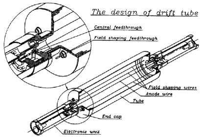
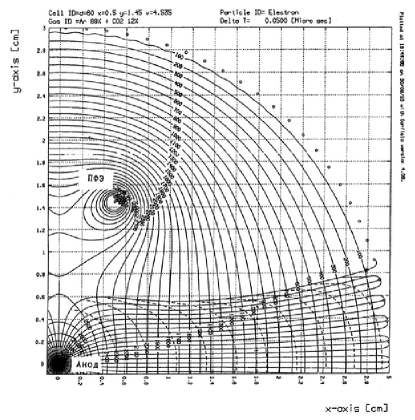
Figure 2: a) The design of the drift tube; b) Calculated electron field lines and equipotentials with a voltage at the anode and the field-shaping wires of 4.5 kV.

4.3 Downstream hodoscopes

The $H_{4X}$ hodoscope located at the entrance to the magnet was made of 10 mm thick scintillator manufactured in Kharkhov (USSR). Dimensions of each of 24 elements seen by PMs from one side were $26\times 400$ mm².

The $H_{5X}$ hodoscope, located downstream of the magnet, was made of 10 mm thick extruded scintillator manufactured in IHEP. The hodoscope consisted of 48 elements of $48\times 1000$ mm² seen by PMs from one side.

The $H_{6X}$ hodoscope situated after the DT system. It was also made of 10 mm thick extruded IHEP manufactured scintillator. There were 32 elements, $65\times 1140$ mm² in size seen by PMs from one side.

The $H_{7}$ hodoscope, located just after the Cherenkov detector Č, had a cell structure. The matrix $8\times 4$ of 20 mm thick scintillation plates of the size $350\times 300$ mm² was geometrically matched with $8\times 4$ mirror matrix inside the Cherenkov detector. Such a system could be used for trigger decisions. The scintillator was manufactured in Kharkov. Each plate was attached to an individual PM.

Following $H_{7}$ the hodoscope $H_{8Y}$ physically consisted of two assemblies placed so that one corresponded to negative and the other one to positive $x$-coordinates with a small overlap (see Fig. 1). That allowed to cover the aperture of 2.8 m in horizontal direction. Each assembly consisted of 32 elements of $48\times 1400$ mm² made of 10 mm thick extruded IHEP manufactured scintillator and seen by PMs from one side. Thus the hodoscope could measure 32 different Y-coordinates and had 64 channels.

All cut surfaces of hodoscope elements were polished. Each element was wrapped with aluminized mylar. All the PMs were of FEU-85 type with the additional magnetic field shielding consisted of multiple layers of Permalloy. Last dinodes of the PMs attached to the central hodoscope elements which were located in the beam region and worked at higher intensity were powered from separate high voltage sources to improve their stability. Signals from PMs were transported via 50 m long $50\,\Omega$ coaxial cables to latches of registering electronics.

5 Cherenkov counters

The system of Cherenkov counters served for the identification of secondary particles and included the RICH velocity spectrometer and hodoscope-like threshold Cherenkov counter Č.

Schematic view of the RICH detector is presented in Fig. 3. The vessel of the detector was made of steel, $150\,{\rm cm}$ long and $70\,{\rm cm}$ in diameter. It consisted of two parts to allow easy access to photodetectors. Entrance and exit flanges were made of $0.8\,{\rm mm}$ aluminum.

Figure 3: Schematic view of the RICH detector (cut in horizontal plane).

Sulfurhexafluoride (${\rm SF}_{6}$), also known as elegas, was used as a radiator. The working pressure was slightly above atmospheric one (up to 10–15%). The typical value of the refractive index was 1.0008, what corresponded to the $\pi/K/p$ threshold momenta of $3.5/12.4/23.6\,{\rm GeV}/c$.

The optical system consisted of 2 identical spherical ($F=125\,{\rm cm}$) glass mirrors of rectangular ($30{\times}35\,{\rm cm}^{2}$) shape. The important features of the detector were that the mirrors were thin ($0.5\,{\rm cm}$) and each mirror focused light into one photomatrix, thus avoiding the need for precise alignment before the run.

Photodetector consisted of 2 photomatrices, each having 23 rows and 16 columns, 736 photo-multipliers in total. Phototubes were hexagonally packed with $1.5\,{\rm cm}$ step (see Fig. 4 for layout). Russian-made FEU-60 phototubes with glass entrance window and $1.0\,{\rm cm}$ photocathode diameter were used. To improve light registration efficiency aluminized mylar cones and wavelength shifters (WLSs) were utilized.

WLSs were made according to the technology developed at IHEP. A thin ($20\,\mu m$) film was covered by the $\simeq 5\,\mu m$ thick transparent layer of p-terphenyl. Circle shape cutouts of such film based WLSs were attached to the FEU-60 entrance windows with an optical grease. The WLSs allowed to utilize the ultraviolet part of Cherenkov light spectrum (which would be otherwise absorbed by glass windows) by shifting it to wavelengths of maximum spectral sensitivity of the PMs. The number of Cherenkov photons emitted per unit wavelength is defined by the formula $dN/d\lambda\propto 1/\lambda^{2}$ which shows that a significant gain can be achieved by using the more intense shortwave part of the spectrum. According to [25, 26] the sensitivity of glass window PMs with p-terphenyl based WLSs can be increased by a factor of 2–3.5. Measurements carried out at IHEP with the $\mathrm{MgF}_{2}$ crystalline radiator, a batch of FEU-60 PMs and the described WLSs showed the increase in the number of photoelectrons by a factor of 2.5.

Figure 4: Layout of the RICH photodetector and example of an event. Mirror alignment (reflection positions of the parallel to detector axis light ray) is shown by the ”+” markers.

Phototubes had operating voltage in the 1–2$\,{\rm kV}$ range. They were powered via resistor chains, which provided the possibility of the voltage adjustment for each tube. Preamplifiers with a sensitivity of 3–5$\,{\rm mV}/\mu{\rm A}$ were attached to the phototubes. Amplified signals were transmitted via $2\,{\rm m}$ long coaxial cables to the discriminators with $10\,{\rm mV}$ threshold, which were located outside the vessel. The discriminators generated differential ECL signals which were transmitted with twisted pairs to the latches of custom-made registering electronics.

The performance characteristics of RICH are given in Table 2 (see [27] for more details on the RICH).

Table 2: The performance characteristics of RICH

Noise level (beam-on)	$\sim 1.5$ hits/trigger
Noise level (beam-off)	$\sim 1$ hits/trigger
Average number of hits per maximum radius ring	10.3
$K$/$\pi$ separation at $2\sigma$ level up to momentum of	30 GeV

The vessel of the multichannel counter Č made of steel was $300$ cm long and $300$ cm in diameter. It housed 32 spherical mirrors of rectangular shape of $350\times 300$ mm² ($8\times 4$ matrix) focusing Cherenkov light to the 32 PMs FEU-39. The counter was filled with air at atmospheric pressure and had threshold momenta for $\pi/K/p$ equal to 6.0/21.3/40.1 GeV/$c$. The counter Č together with the hodoscope $H_{7}$ (the matrix of the same size) allowed to construct simple particle identification requirements which could be used in the trigger.

6 Electromagnetic calorimeter

A multichannel lead glass electromagnetic calorimeter (ECAL) had been previously used in the EHS experiment at CERN [28] (known as Intermediate Gamma Detector there). It had a standard design of a two-dimensional lead glass matrix which allowed to measure both the position and the energy of a shower.

The initial assembly was rearranged to reduce the originally big central hole to the size of one counter. The hole was still needed to let the beam pass through. The ECAL array of $39\times 27-1$ counters covers a surface of $1.95\times 1.35$ m² (horizontal$\times$vertical). The individual counters with dimensions $5\times 5\times 42$ cm³ were made of lead glass F8 manufactured in USSR, with radiation length $X_{0}=2.8$ cm. The ECAL was mounted on a movable two-coordinate platform so that each counter could be calibrated individually by exposing it to an electron beam.

The PMs (FEU-84) were shielded individually against the magnetic field of the order of 20 G. The shielding consisted of cylinders of “steel-50” and Permalloy.

A new monitoring system was built for ECAL consisting of four LED sources and a light distribution system which had light guides coming individually to the front of each lead glass counter.

The typical energy and position resolutions obtained with an electron beam were $\frac{\Delta E}{E}=\frac{0.15}{\sqrt{E/{\rm GeV}}}+0.02$ (FWHM) and $\sigma\simeq\frac{8.2~{}{\rm mm}}{\sqrt{E/{\rm GeV}}}$ correspondingly.

7 Hadron calorimeter

A hodoscopic hadron calorimeter can be thought of as a $12\times 8$ matrix of full absorption counters of $20\times 20$ cm². The calorimeter aperture was $2.5\times 1.6$ m², the total weight was 30 t. Actually an independent element of the calorimeter was an assembled still container housing four counters each consisted of 80 plates of 20 mm thick steel ($\approx 5$ nuclear interaction lengths) with interlayers of plastic scintillator plates, 5 mm thick. The light was collected by means of wavelength shifting light-guides seen from one side by PMs FEU-110.

The energy resolution for hadrons in the energy range $E=4$–$40$ GeV was $\sigma_{E}/E=0.02+0.52/\sqrt{E}$ where $E$ is in GeV and the mean space resolution was $\approx 2$ cm at 40 GeV.

More information on the hadron calorimeter can be found in [29].

8 Trigger

The two-level trigger scheme was used with the SPHINX facility (to reduce DAQ system dead time). At zero level so called strobe signals were generated. There were three different strobe signals described by the logical formulae:

$$T_{0}^{b} = S_{1}S_{2}S_{3}S_{4}\cdot(\overline{B_{1}B_{2}})\cdot\overline{A_{5-8}}\cdot Gate\cdot\overline{Busy},$$ (1)

$$T_{0}^{c} = S_{1}S_{2}S_{3}S_{4}\cdot(\overline{B_{1}B_{2}})\cdot Gate\cdot\overline{Busy},$$ (2)

$$T_{0}^{d} = S_{1}S_{2}S_{3}S_{4}\cdot Gate\cdot\overline{Busy}\cdot Prescale,$$ (3)

Their logical “OR” was one of the input signals for the next level trigger. The $Gate$ was synchronized with the “begin of spill” signal, the $Busy$ was used to prevent generating $T_{0}$ for the time the decision was being made by the next level trigger and possible subsequent readout cycle, the $Prescale$ was the signal from the prescaling generator reducing the original rate of this strobe by a factor of $\simeq 16000$.

The block of the first level trigger logic allowed to generate up to eight signals using as primitive elements information from scintillation and veto counters, multiplicity of hits in the hodoscopes and the threshold Cherenkov counter and total energy sum in the ECAL. It also produced the logical “OR” of the above signals which served as a “general” trigger and started event readout.

The vast majority of the collected statistics corresponded to so called three-track trigger

$$T_{(3)}=T_{0}^{b}\cdot H_{3}(0{-}1)\cdot H_{4}(2{-}3)\cdot H_{6}({\equiv}3)\cdot H_{7}(1{-}3),$$ (4)

where $H_{i}(m_{1}{-}m_{2})$ means multiplicity requirement between $m_{1}$ and $m_{2}$ in hodoscope $H_{i}$. It allowed to select events with three charged tracks in the final state produced in exclusive reactions. Other important triggers used during data taking runs are listed below:

$$T_{(5)}=T_{0}^{b}\cdot H_{3}(0{-}1)\cdot H_{4}(4{-}5)\cdot H_{5}({\geqslant}4)\cdot H_{6}({\equiv}5)\cdot H_{7}(3{-}6)$$ (5)

or five-track trigger allowed to select exclusive reactions with five secondary tracks;

$$\begin{array}[]{rcl}T_{(2)}&=T_{0}^{c}\cdot(&\!H_{3}({\geqslant}1)\cdot H_{4}(1{-}2)\cdot H_{5}(2{-}3)\cdot H_{6}({\equiv}2)\cdot H_{7}({\equiv}2)\ +\\ &&\!H_{3}({\geqslant}1)\cdot H_{4}(2{-}3)\cdot H_{5}(2{-}4)\cdot H_{6}({\equiv}3)\cdot H_{7}(2{-}3)\ )\end{array}$$ (6)

or “meson” trigger selected inclusive reactions with two or tree charged tracks in the final state;

$$T_{(neu)}=T_{0}^{c}\cdot H_{3}({\geqslant}1)\cdot H_{5}({\equiv}0)\cdot H_{6}({\equiv}0)\cdot H_{7}({\equiv}0)\cdot E_{\rm ECAL}>0$$ (7)

or neutral trigger selected events with only neutral secondary particles and some energy deposited in the ECAL ($E_{\rm ECAL}>0$);

$$T_{(beam)}=T_{0}^{d}$$ (8)

or beam trigger — prescaled trigger on a beam particle.

All these trigger signals could be used simultaneously. In reality, different subsets of them were used during different periods of data taking runs. This allowed to select many exclusive reactions and calibration processes, part of which will be discussed in section 11.

9 DAQ hardware

DAQ architecture was based on IHEP developed MISS standard [30]. Some modules were in IHEP SUMMA standard [31]. The system topology had four-level structure:

1. Front-end electronics level (lowest one) included modules of latches, TDCs and ADCs as well as crate controllers and special module controllers. All modules were of either MISS or SUMMA types.

2. Branch buffer memory level served as an intermediate storage of event information from a single branch and for partial event building. All modules were of MISS type.

3. System buffer memory level served as an intermediate storage of event information from the whole system and for event building. Its design was similar to the branch buffer memory level.

4. Data accumulation level (spill data level) built a packet containing information on all events happened during one spill. In addition, apparatus control and monitoring functions were performed at this level.

Table 3 gives the numbers of channels used to record physical information for the SPHINX setup arranged by module type.

Table 3: Channels of SPHINX setup arranged by the front-end module type

Type	Detector	Number of channels
ADC	HCAL, ECAL	$\sim$ $1400$
TDC	DT	$\sim$ $\,\ 700$
Latches	PC, hodoscopes, RICH	$\sim$ $5000$
Total		$\sim$ $7100$

All inter-level connections were also designed according to MISS specifications. More information on the electronics used in the system can be found in [32, 33, 34, 35].

The general scheme of the SPHINX DAQ system is shown in Fig. 5. The lowest (first) level had 25 sectors of registering electronics. Each sector of the second level was connected to $2$–$9$ first level sectors to keep data flow at the optimum level. The system could use SUMMA crates as MISS sectors at the first level. Additional special controllers in such crates simulated standard MISS controllers. These SUMMA crates contained modules of a trigger logic.

The working algorithm was fully based on standard MISS procedures. The “begin of spill” signal started a reset cycle. Event selection was done in two stages with generating of strobe signals and trigger signals at the first and the second stage correspondingly. A set of strobe signals was produced by a strobe-block and an auxiliary logic fed by information from the beam counters and the guard system. The logical “OR” of these signals allowed registering information from hodoscopes, PC and RICH (all latches). It also put the strobe-block into a busy state preventing it from generating further strobes. The information on strobe type, multiplicity in the particular set of hodoscopes and on energy deposited in the ECAL came to a trigger block [36] where the final decision on whether to accept an event or not was made. If it was negative, the fast reset signal was distributed to the activated part of the electronics followed by clearing the strobe-block busy state. If positive, the information from the ECAL, the HCAL and the DT was registered. This signal also initiated the process of the front-end electronics readout and moving the data to the next level. This was accompanied by extending the strobe/trigger logic busy state for the time of the readout. When done the busy state was cleared and the system was ready for further data taking. As the data collection proceeded, the information moved up through the intermediate levels and was accumulated at the top level.

Thus, given that the “begin of spill” signal was provided, the hardware part of the DAQ system was capable to collect, build and store the information on the events collected during the spill according to trigger types programmed into the trigger block without any outside intervention. This information was stored in the 16 MB buffer memory module of the top level VME crate.

The “begin of spill” signal was provided by a software. The software also generated additional trigger signals of special types for calibration data collection and saved all the collected data to a permanent storage media.

Some basic DAQ characteristics are given in the Table 4.

Table 4: Characteristics of the SPHINX DAQ system

spill/cycle time 1.5 sec/9 sec trigger rate 4 KHz event length 1.3 KByte data flow 5.2 MByte/sec live time $\sim 70\%$

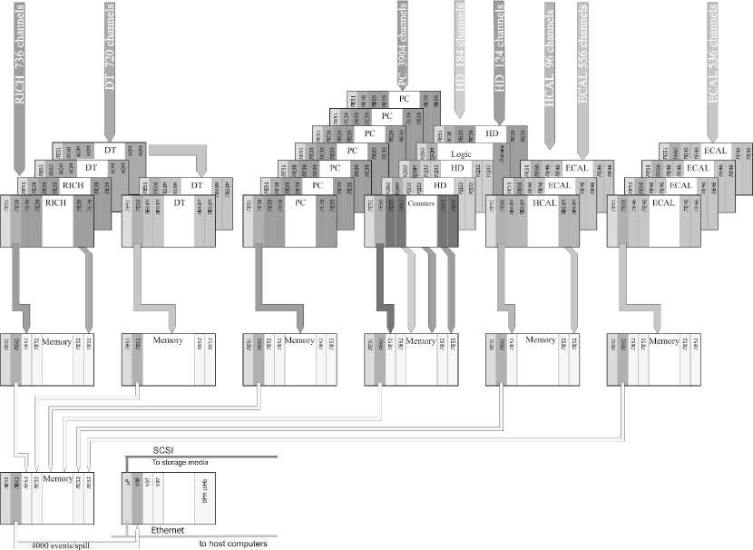
Figure 5: Scheme of the DAQ of the SPHINX setup

10 DAQ and online software

The DAQ software provided the following functions: start/stop of the basic data collection mode (which includes calibration data collection), writing the collected data to disks and/or magnetic tapes, online apparatus monitoring, initiating special modes for apparatus and DAQ tests and calibrations.

The DAQ software worked mostly under LynxOS operating system installed on a one-board MVME-167 computer with Motorola-68040 CPU and 16 MB of memory. The computer was located in the top level VME crate. The top level memory buffer (also 16 MB) located in the same crate was mapped to the computer memory address space so that it could be accessed by the processor as a part of its own memory.

The software design allowed to distribute a part of the event flow (including the whole) to consumers on other computers via Ethernet. The online monitoring worked this way so that apparatus control parameters could be analyzed with two workstation (DECStation 5200 and Silicon Graphics Indy) working under UNIX-type OS.

The software had the following modules (programs):

1. a dispatcher managing the whole system;

2. data collection modules;

3. disks/tapes writing modules;

4. data distributor;

5. DAQ test and control modules;

6. apparatus test and calibration modules.

The dispatcher was the core of the system. It accepted messages from the connecting modules and communicated them to other modules according to the type of the sending module and the message content for actions.

The data collection modules consisted of the main program working on in-spill information and auxiliary programs which were not necessarily spill-tied. The main program activated by the “begin of spill” signal (coming from an accelerator control apparatus), initialized the DAQ apparatus and initiated three special sequences: for pedestal measurements, for collecting data with the ECAL and the RICH monitoring systems, for collecting TDC calibration data. By the “end of spill” signal it also sent the message with parameters of the collected data buffer to the dispatcher thus making this information available for other modules. Another data collection module read out scalers. The reading sequence started by the end of the spill. The collected information then was communicated (through the dispatcher) for writing to disks and for displaying the scalers readings.

The data could be written to disk files which could be then written to tapes or directly to tapes (an Exabyte drive was attached to the MVME-167).

There was the distributing module which could send out the information on the uniform subset of events via Ethernet. This was used for the online apparatus monitoring. On the other side (workstations) the information was further distributed to different analyzing processes (analyzers). It was done in the framework of UNIDAQ system [37, 38]. One of the advantages of this system was that analyzers were different programs which had a standard piece of code allowing them to connect to the central distributing unit (NOVA) and got the data. Thus they could be written by different people for different purposes. There were analyzers for filling and displaying control histogram, for single event display, for online chamber efficiency measurements with tracks, for testing the structure of events built by electronics, for monitoring recoverable electronic failures. Another special analyzer monitored some, presumably constant, setup parameters and produced an information message on a main console accompanied by an alarm signal if these parameters came out of predefined windows.

The DAQ system could be controlled by sending messages to different modules or to all modules at once with the special program. There was a set of programs for the DAQ hardware testing and debugging and also for the apparatus testing and calibrations.

11 Illustration of the experimental possibilities

In this section we will consider very briefly several possibilities for the measurements with the SPHINX facility with different triggers.

$\bf T_{(3)}$ trigger

The three-track trigger $T_{(3)}$ (4) was the main trigger for the measurement with the SPHINX spectrometer. It allowed to study simultaneously the exclusive reactions:

$$p+N({\rm C}) \to [pK^{0}_{L}]K^{0}_{S}+N({\rm C});\ K^{0}_{S}\to\pi^{+}\pi^{-}$$ (9)

$$\to [nK^{+}]K^{0}_{S}+N({\rm C});\ K^{0}_{S}\to\pi^{+}\pi^{-}$$ (10)

$$\to pK^{+}K^{-}+N({\rm C})$$ (11)

$$\to pK^{0}_{S}K^{0}_{L}+N({\rm C});\ K^{0}_{S}\to\pi^{+}\pi^{-}$$ (12)

$$\to p\phi+N({\rm C});\ \phi\to K^{+}K^{-},\ K^{0}_{S}K^{0}_{L}$$ (13)

$$\to \Lambda K^{+}+N({\rm C});\ \Lambda\to p\pi^{-}$$ (14)

$$\to [\Sigma^{0}K^{+}]+N({\rm C});\ \Sigma^{0}\to\Lambda\gamma;\ \Lambda\to p\pi^{-}$$ (15)

$$\to [\Sigma^{+}K^{0}_{S}]+N({\rm C});\ K^{0}_{S}\to\pi^{+}\pi^{-};\ \Sigma^{+}\to p\pi^{0},\ n\pi^{+}$$ (16)

$$\to \Lambda(1520)K^{+}+N({\rm C});\ \Lambda(1520)\to pK^{-},\ \Lambda\gamma;\ \Lambda\to p\pi^{-}$$ (17)

and many other processes (reactions on quasi-free nucleons $N$ or coherent reactions on $C$ nuclei). The long lived neutral particles ($n$, $K^{0}_{L}$, $\gamma$) were detected by their interactions in the ECAL calorimeter and were not used in the trigger requirements.

$\bf T_{(5)}$ trigger

The five-track trigger $T_{(5)}$ (5) was used, for example, for the selection of reactions:

$$p+N({\rm C}) \to [pK^{0}_{S}]K^{0}_{S}+N({\rm C});\ K^{0}_{S}\to\pi^{+}\pi^{-}$$ (18)

$$\to \Lambda(1520)K^{+}+N({\rm C});\ \Lambda(1520)\to\Lambda\pi^{+}\pi^{-};\ \Lambda\to p\pi^{-}$$ (19)

$\bf T_{(2)}$ and $\bf T_{(neu)}$ triggers

These triggers (6) and (7) were used for the study of quasi-exclusive forward meson production in proton reactions in deep fragmentation region (inclusive for bottom vertex) [11]:

$$p+N\to(meson)|_{\rm forward}+(X)|_{\rm bottom\ vertex}$$ (20)

These deep fragmentation processes can be accompanied by substantial quark rearrangement, gluon forward bremsstrahlung and open new possibilities for the search for exotic meson production [39].

The possibilities to select some of the above reactions are illustrated in Fig. 7–7 reproduced from [17]. Reactions (9), (10), (18) were used for the search for the exotic pentaquark baryon $\Theta(1540)^{+}$ with positive strangeness and $uudd\bar{s}$ quark structure in the mass spectra of $[nK^{+}]$, $[pK^{0}_{S}]$, $[pK^{0}_{L}]$ systems [17]. Reactions (15), (16) were used for the search for the cryptoexotic $X(2000)$ baryon with hidden strangeness ($uuds\bar{s}$) in the mass spectra $M(\Sigma^{0}K^{+})$ and $M(\Sigma^{+}K^{0}_{S})$ [3, 6, 8, 9, 12, 13, 16].

The SPHINX facility had the good guard system allowing to suppress background processes with “lost photons”. That opened the possibility to study the rare radiative decay $\Lambda(1520)\to\Lambda\gamma$ in the reaction (17) — see Fig. 8 reproduced from [18].

12 Conclusion

The multipurpose wide-aperture SPHINX spectrometer, in its several modifications, was used in the experiments at the proton beam of IHEP U-70 accelerator in 1989–1999 [1–18]. The good quality of this setup with the possibility of the complete reconstruction of charged and neutral secondary particles and large collected statistics allowed to get many results on the study of diffractive production reactions, searches for new states of hadronic matter, study of the radiative decays of hyperons, OZI rule and deep fragmentation reactions [1–18] and opened new perspectives for further investigations of these and other rare processes.

Figure 6: Signals from decays of $K_{S}^{0}\to\pi^{+}\pi^{-}$ and $\Lambda\to p\pi^{-}$ in the reactions $p+N\to nK_{S}^{0}K^{+}+N$ and $p+N\to\Lambda\pi^{+}\pi^{-}K^{+}+N$. The fit gives: $M(K_{S}^{0})=496$ MeV, $\sigma(K_{S}^{0})=8.4$ MeV, $M(\Lambda)=1116$ MeV, $\sigma(\Lambda)=3.8$ MeV (see [17]).

Figure 7: Effective mass distributions $M(pK^{-})$, $M(nK_{S}^{0})$ for the reaction $p+N\to[N\bar{K}]K^{+}+N$ (two left pictures), and $M(K^{+}K^{-})$, $M(K_{S}^{0}K_{L}^{0})$ for the reaction $p+N\to p[K\bar{K}]+N$ (two right ones; see [17]).

Figure 8: Effective mass spectrum $M(\Lambda\gamma)$ in reaction $p+N({\rm C})\to[\Lambda\gamma]K^{+}+N({\rm C});\ \Lambda\to p\pi^{-}$. The arrow shows the $\Lambda(1520)$ peak. The right-top picture presents the same spectrum obtained with more stringent criteria for suppression of extra photons [18].

References

- [1] D. V. Vavilov et al. (SPHINX Collab.), Yad. Fiz. 57, 241 (1994) [Phys. At. Nucl. (Engl. Transl.) 57, 227 (1994)]; M. Ya. Balatz et al. (SPHINX Collab.), Z. Phys. C 61, 220 (1994).
- [2] M. Ya. Balatz et al. (SPHINX Collab.), Z. Phys. C 61, 399 (1994).
- [3] D. V. Vavilov et al. (SPHINX Collab.), Yad. Fiz. 57, 253 (1994) [Phys. At. Nucl. (Engl. Transl.) 57, 238 (1994)].
- [4] L. G. Landsberg et al. (SPHINX Collab.), Nuov. Cim. A 107, 2441 (1994).
- [5] D. V. Vavilov et al. (SPHINX Collab.), Yad. Fiz. 57, 1449 (1994); 58, 1426 (1995) [Phys. At. Nucl. (Engl. Transl.) 57, 1376 (1994); 58, 1342 (1995)].
- [6] S. V. Golovkin et al. (SPHINX Collab.), Z. Phys. C 68, 585 (1995).
- [7] S. V. Golovkin et al. (SPHINX Collab.), Yad. Phys. 59, 1395 (1996) [Phys. At. Nucl. (Engl. Transl.) 59, 1336 (1996)].
- [8] V. A. Bezzubov et al. (SPHINX Collab.), Yad. Phys. 59, 2199 (1996) [Phys. At. Nucl. (Engl. Transl.) 59, 2117 (1996)].
- [9] L. G. Landsberg, Hadron Spectroscopy (”Hadron 97”). Seventh Intern. Conf. Upton, NY, Aug. 1997 (Ed. S.-U. Chung, H. J. Willutzki), p. 725.
- [10] V. A. Victorov et al., Yad. Fiz. 59, 1229 (1996) [Phys. At. Nucl. (Engl. Transl.) 59, 1175 (1996)]; M. Ya. Balatz et al. (SPHINX Collab.), Yad. Fiz. 59, 1242 (1996) [Phys. At. Nucl. (Engl. Transl.) 59, 1186 (1996)]; S. V. Golovkin et al. (SPHINX Collab.), Z. Phys. A 359, 435 (1997).
- [11] S. V. Golovkin et al. (SPHINX Collab.), Z. Phys. A 359, 327 (1997).
- [12] S. V. Golovkin et al. (SPHINX Collab.), Eur. Phys. J. A 5, 409 (1999).
- [13] D. V. Vavilov et al. (SPHINX Collab.), Yad. Fiz. 63, 1469 (2000).
- [14] L. G. Landsberg, Phys. Rep. 320, 223 (1999); L. G. Landsberg, Yad. Fiz. 62, 2167 (1999).
- [15] L. G. Landsberg, UFN 164, 1129 (1994) [Physics Uspekhi (Engl. Transl.) 37, 1043 (1994)]; V. F. Kurshetsov, L. G. Landsberg, Yad. Fiz. 57, 2030 (1994) [Phys. At. Nucl. (Engl. Transl.) 57, 1954 (1994)]; L. G. Landsberg, Yad. Fiz. 60, 1541 (1997) [Phys. At. Nucl. (Engl. Transl.) 60, 1397 (1997)].
- [16] Yu. M. Antipov et al. (SPHINX Collab.), Yad. Fiz. 65, 2131 (2002) [Phys. At. Nucl. (Engl. Transl.) 65, 2070 (2002)].
- [17] Yu. M. Antipov et al. (SPHINX Collab.), Eur. Phys. J. A 21, 455 (2004); V.F. Kurshetsov et al. (SPHINX Collab.), Yad. Fiz. 68, 468 (2005) [Phys. At. Nucl. (Engl. Transl.) 68, 439 (2005)].
- [18] Yu. M. Antipov et al. (SPHINX Collab.), Phys.Lett. B 604, 22 (2004); D. V. Vavilov et al. (SPHINX Collab.), Yad. Fiz. 68, 407 (2005) [Phys. At. Nucl. (Engl. Transl.) 68, 378 (2005)].
- [19] A.A. Batalov et al., Preprint IFVE-87-116 (1987) (in Russian).
- [20] A.V. Vishnevsky et al., Prib. Tekh. Eksp. 1, 60 (1984) (in Russian).
- [21] Yu. Antipov et al., Nucl. Instr. and Meth. in Phys. Res. A 379, 434 (1996).
- [22] S. Zimin, M. Soldatov, Preprint IFVE-93-50 (1993) (in Russian).
- [23] Yu. Antipov et al., Nuclear Physics B (Proc. Suppl.) 44, 206 (1995).
- [24] Yu. Antipov et al., Preprint IFVE-94-128 (1994) (in Russian).
- [25] A.M. Gorin et al., Nucl. Instr. Meth. A 251, 461 (1986).
- [26] P. Baillon et al., Nucl. Instr. Meth. 126, 13 (1975).
- [27] A. Kozhevnikov, V. Kubarovsky, V. Molchanov, V. Rykalin and V. Solyanik, Nucl. Instr. Meth. A 433, 164 (1999).
- [28] B. Powell et al., Nucl. Instr. Meth. 198, 217 (1982).
- [29] Y.M. Antipov et al., Nucl. Instr. Meth. A 295, 81 (1990).
- [30] S.I. Bityukov et al., Preprint IFVE-94-101 (1994) (in Russian).
- [31] O.I. Alferova et al., Prib. Tekh. Eksp. 4, 56 (1975) (in Russian).
- [32] Yu. Bushnin et al., Preprint IFVE-88-47 (1988) (in Russian).
- [33] Yu. Bushnin et al., Preprint IFVE-93-72 (1993) (in Russian).
- [34] Yu. Bushnin et al., Preprint IFVE-95-88 (1995) (in Russian).
- [35] Yu. Bushnin et al., Preprint IFVE-95-104 (1995) (in Russian).
- [36] A. Kozhevnikov et al., Preprint IFVE-91-101 (1991) (in Russian).
- [37] M. Nomachi et al. Proceedings of the International Conference on Computing in High-energy Physics (CHEP 94), LBL-35822, 114 (1994).
- [38] UNIDAQ collaboration, SDC-93-573 (1993); UMHE-93-29 (1993).
- [39] L.G. Landsberg, Yad. Fiz. 52, 192 (1990); Nucl. Phys. (Proc. Suppl.) 211, 179 (1991).