Scaling collapse and structure functions: Identifying self-affinity in finite length time series.

Zusammenfassung

Empirical determination of the scaling properties and exponents of time series presents a formidable challenge in testing, and developing, a theoretical understanding of turbulence and other out-of-equilibrium phenomena. We discuss the special case of self affine time series in the context of a stochastic process. We highlight two complementary approaches to the differenced variable of the data: i) attempting a scaling collapse of the Probability Density Functions which should then be well described by the solution of the corresponding Fokker-Planck equation and ii) using structure functions to determine the scaling properties of the higher order moments. We consider a method of conditioning that recovers the underlying self affine scaling in a finite length time series, and illustrate it using a Lévy flight.

Theories of turbulence as applied to single point measurements in a flow concern the scaling properties, in a statistical sense, of differenced time series, where the Taylor hypothesis is invoked so that the difference between measurements at some time $t$ and a later time $t+\tau$ acts as a proxy for the difference between measurements made at two points in the fluid separated by length scale $L$. Studies of scaling in solar wind turbulence have focused on the power spectra and the structure functions (see e.g. [Tu and Marsch, (1995), Horbury and Balogh(1997)]) and, more recently, the Probability Density Function (PDF) ([Hnat et al.(2002), Hnat et al.(2003b)]).

The statistical scaling properties of time series can in general, however, be considered in a similar manner. There is a considerable literature concerning scaling in auroral region magnetometers and in geomagnetic indices (such as [Tsurutani et al.(1990), Takalo et al.(1993), Consolini et al.(1996), Vörös et al.(1998), Uritsky and Pudovkin(1998), Watkins et al.(2001), Kovács et al.(2001)]). This is motivated in part by attempts to understand the driven magnetospheric system from the perspective of scaling due to intrinsic processes (see e.g. [Chapman and Watkins(2001)] and references therein) and their relationship to that of the turbulent solar wind driver. This necessitates quantitative comparative studies of scaling in time series (e.g. [Takalo and Timonen(1998), Freeman et al.(2000), Uritsky et al.(2001), Vörös et al.(2002), Hnat et al.(2003a)]). Such studies can to some extent fruitfully consider the low order moments, whereas a particular difficulty for comparison of observations with models of turbulence is that the intermittency parameter in turbulence $\tau(2)$ is determined by the $6^{th}$order structure function [Frisch(1995)].

More recently, studies have focussed on the scaling properties and functional form of the PDFs of the differenced time series (see e.g. [Consolini and De Michelis(1998), Sorriso-Valvo et al (2001), Weigel and Baker(2003a), Stepanova et al.(2003)]). This leads to a Fokker-Planck model in the case of self- similarity ([Hnat et al.(2003b), Hnat et al. (2005)]).

In this paper we describe an approach to modelling such scaling data which exploits the data’s self-affine property by applying the idea of coarse graining the data ([Wilson (1979), Sornette(2000)]), here, in the time domain. This coarse-graining can be achieved empirically, from the data, by a scaling collapse procedure (e.g.[Hnat et al.(2003b), Hnat et al. (2005)]) (section 2), and, then having experimentally determined the scaling exponent, we can take the approach one stage further and seek to describe the data by means of a particular case of a generalised Fokker-Planck equation (GFPE, section 5). We stress here that the GFPE is here, as elsewhere (eg [Sornette(2000)]), applied to a much more general class of problem than the strictly equilibrium physics for which the original FPE was obtained. The GFPE represents an alternative to the fractional Fokker-Planck equation (e.g. [Zaslavsky (1995)]) which is also applicable in such non-equilibrium cases.

The critical steps in this process are then (i) establishing whether a given dataset is self affine and (ii) determining the scaling exponent. We highlight two important issues that arise in the analysis of physical datasets here.

The first of these is that SDE models for the data, and indeed, coarse graining, deal with the properties of an arbitrarily large dataset. We use a well understood example of a self affine timeseries, that of ordinary Levy motion (section 3), to show how conditioning of the data is needed to recover the known scaling of an arbitrarily large timeseries from one finite length. We then use an example of a naturally occurring timeseries, that of the AE geomagnetic index, shown previously to exhibit self affine scaling over a range of timescales, to highlight the effectiveness, and the limitations, of this technique.

The second of these is that knowledge of the scaling properties of (in principle all) the non zero moments is needed to capture the scaling properties of a timeseries. We again use the AE timeseries to illustrate this point by constructing a fractional Brownian motion fBm with the same second moment, but with a very different PDF.

1 Self affine time series: concepts

From a time series $x(t)$ sampled at times $t_{k}$, that is at evenly spaced intervals $\Delta=t_{k}-t_{k-1}$ we can construct a differenced time series with respect to the time increment $\tau=s\Delta$:

$$y(t,\tau)=x(t+\tau)-x(t)$$ (1)

so that

$$x(t+\tau)=x(t)+y(t,\tau)$$ (2)

If we consider $N$ successive values determined at intervals of $\Delta$, that is, $y(t_{1},\Delta)..y(t_{k},\Delta)...y(t_{N},\Delta)$, their sum gives:

$$x(t)=\sum_{1}^{N}y(t_{k},\Delta)+x_{0}$$ (3)

where $x_{0}=x(t-N\Delta)$. As $N\rightarrow\infty$ the sum (3) of the $y$ tends to the original time series $x(t)$.

We will make two assumptions: i) that the $y(t,\tau)$ is a stochastic variable so that (2) can be read as a random walk and ii) that the $y$ are scaling with $\tau$ (to be defined next).

By summing adjacent pairs in the sequence, for example:

$$y^{(1)}(t_{1},2\Delta)=y(t_{1},\Delta)+y(t_{2},\Delta)$$ (4)

one can coarsegrain (or decimate) the time series in $\tau$. This operation gives the $x(t)$ as a random walk of $N/2$ values of $y$ determined at intervals of $\tau=2\Delta$. We can successively coarsegrain the sequence an arbitrary number of times:

$$x(t) = y(t_{1},\Delta)+y(t_{2},\Delta)+\cdots+y(t_{k},\Delta)+y(t_{k+1},\Delta)+\cdots+y(t_{N},\Delta)$$

$$= y^{(1)}(t_{1},2\Delta)+\cdots+y^{(1)}(t_{k},2\Delta)+\cdots+y^{(1)}(t_{N/2},2\Delta)$$

$$= y^{(n)}(t_{1},2^{n}\Delta)+\cdots+y^{(n)}(t_{k},2^{n}\Delta)+\cdots+y^{(n)}(t_{N/2^{n}},2^{n}\Delta)$$

where this procedure is understood in the renormalization sense in that both $N$ and $n$ can be taken arbitrarily large, so that a timeseries of arbitrarily large length is considered. This procedure can apply to a finite sized physical system of interest provided that that system supports a large range of spatio- temporal scales (the smallest being $\Delta$, the largest, $2^{n}\Delta$, $n$ large), an example of this is the inertial range in fluid turbulence.

We now consider a self affine scaling with exponent $\alpha$:

$$y^{\prime}=2^{\alpha}y,\;\;\;\tau^{\prime}=2\tau,$$ (6)

so that

$$y^{(n)}=2^{n\alpha}y,\;\;\;\tau=2^{n}\Delta$$ (7)

For arbitrary $\tau$ we can normalize ($\tau\equiv\tau/\Delta$) and write

$$y^{\prime}(t,\tau)=\tau^{\alpha}y(t,\Delta)$$ (8)

Now if the $y$ is a stochastic variable with self affine scaling in $\tau$, there exists a self similar PDF which is unchanged under the transformation (8):

$$P(y^{\prime}\tau^{-\alpha})\tau^{-\alpha}=P(y)$$ (9)

Importantly, the $y^{\prime}s$ are not necessarily Gaussian distributed stochastic variables, but do possess self similarity as embodied by (9).

This property is shared by the ($\alpha-$stable) Lévy flights ([Shlesinger et al, (1995)]) for $N\rightarrow\infty$. The special case where the $y^{\prime}s$ are both independent, identically distributed (iid) and have finite variance corresponds to a Brownian random walk. One can show directly from the above renormalization (see for example [Sornette(2000)]) that the Brownian case is just the Central Limit Theorem with $\alpha=1/2$ and Gaussian $P(y)$. Here, we consider time series which possess the properties (8) and (9), which may have $\alpha\neq 1/2$ and which are time stationary solutions of a Fokker-Planck equation.

An important corollary of (9) is of the scaling of the structure functions (and moments). The $p^{th}$ moment can be written as:

$$m_{p}=<y^{p}>=\int_{-\infty}^{\infty}P(y)y^{p}dy=\tau^{p\alpha}\int_{-\infty}^{\infty}P(y^{\prime})y^{\prime p}dy^{\prime}$$ (10)

so that

$$m_{p}\sim\tau^{p\alpha}$$ (11)

via (9).The scaling of any of the non zero moments of a self affine time series is thus sufficient to determine the exponent. Importantly, all the non zero moments will share this same scaling. This can also be appreciated directly by writing the PDF as an expansion in the moments. If we define the Fourier transform of the PDF $P(z)$ of a given time series $z(t)$ by:

$$\hat{P}(k)=\int_{-\infty}^{\infty}e^{ikz}P(z)dz$$ (12)

then it is readily shown that the $p^{th}$ moment is given by:

$$m_{p}=(-i)^{p}\frac{d^{p}\hat{P}(k)}{dk^{p}}\mid_{k=0}$$ (13)

where $d^{p}/dk^{p}$ denotes the $p^{th}$ derivative with respect to $k$. From this it follows that the PDF can be expressed as an expansion in the moments:

$$\hat{P}(k)=\sum_{p=0}^{\infty}\frac{m_{p}}{p!}(ik)^{p}$$ (14)

Hence the PDF is defined by knowledge of all the non zero moments.

2 Testing for self affine scaling.

2.1 Extracting the scaling of a surrogate, a finite length Lévy flight.

We now discuss methods for testing for the property (9) and measuring the exponent $\alpha$ for a given finite length time series. For the purpose of illustration we consider a Lévy flight of index $\mu=1.8$ which is generated from iid random deviates by the following algorithm for the increments (the $y^{\prime}s$, see [Siegert and Friedrich, (2004)] for details):

$$f_{\mu}=\frac{\sin(\mu r)}{(\cos(r))^{\frac{1}{\mu}}}\left(\frac{\cos[(1-\mu)r]}{v}\right)^{\frac{(1-\mu)}{\mu}}$$ (15)

where $r$ is a uniformly distributed random variable in the range $[-\pi/2,\pi/2]$ and $v$ is an exponentially distributed random variable with mean $1$ which is independent of $r$. The scaling exponent $\alpha$ from (8) and (9) is then related to the Lévy index, $\mu$, by $\alpha=1/\mu$.

One can first consider directly attempting a scaling collapse in the sense of (9), of the PDF of differences obtained over a wide range of $\tau$ (see [Mantegna and Stanley(1995), Hnat et al.(2003a), Hnat et al.(2003b)] for examples). This corresponds to a renormalization of the data as discussed above. We first determine the scaling exponent $\alpha$ from one or more of the moments via (11) or an estimate thereof. In a finite length time series, one would ideally use the scaling of the peak $P(y=0,\tau)$ (that is, the $p=-1$ moment) with $\tau$ as this is better resolved statistically than the higher order moments. In practice however the time series $y(t,\tau)$, formed from the differences of a measured quantity, can as $y\rightarrow 0$ be dominated by observational uncertainties.

Figure 1 shows the scaling collapse (9) applied to a numerically generated Lévy flight (15) of $10^{6}$ increments. The curves correspond to differences at values of $\tau=m\Delta$ with $m=[6,10,16,26,42]$. Error bars denote an estimate of the expected fluctuation per bin of this histogram based on Gaussian statistics (a more sophisticated method for estimating these for the Lévy case may be found in [Siegert and Friedrich, (2004)]). We see that scaling collapse can be verified to the precision with which the PDF is locally determined statistically.

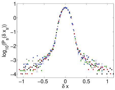
Abbildung 1: Scaling collapse of the PDF of an $\mu=1.8$ Lévy flight.

The exponent $\alpha=0.544$ used to achieve the scaling collapse in Figure 1 was determined empirically directly from an analysis of this finite length time series based on the structure functions discussed below.

As discussed above, the scaling exponent $\alpha$ that successfully collapses the PDF of different $\tau$ should emerge from the scaling of the moments. This is often obtained via the generalized structure functions (see e.g. [Tu and Marsch, (1995), Horbury and Balogh(1997), Hnat et al.(2003a), Hnat et al. (2005)] for examples)

$$S_{p}(\tau)=<|y(t,\tau)|^{p}>\propto\tau^{\zeta(p)}$$ (16)

where for self affine $y(t)$, we have $\zeta(p)=p\alpha$ (for a multifractal, $\zeta(p)$ is approximately quadratic in $p$). From (11) the moments will in principle share this scaling provided that the moment is non- zero (however in a noisy signals a moment that should vanish will be dominated by the noise). In principle we can obtain $\alpha$ from the slopes of log- log plots of the $S_{p}$ versus $\tau$ for any $p$; in practice this is severely limited by the finite length of the dataset.

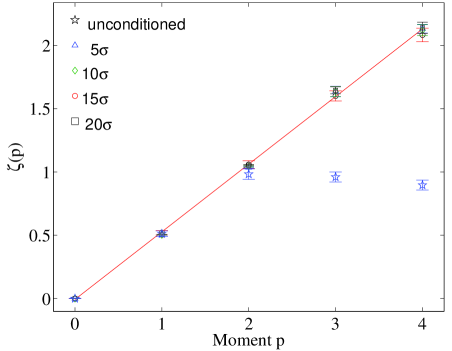
Abbildung 2: The effect of conditioning a Levy flight. $\bigstar$ are the $\zeta(p)$ obtained from the raw time series, all other symbols refer to conditioned time series for different values of $Q$ (see text). The conditioned results yield a scaling exponent $\alpha=0.544$ which corresponds to a Levy index of $\mu=1.84$.

The $\zeta(p)$ for the above Lévy flight obtained via (16) are shown plotted versus $p$ in Figure 2. On such a plot we would expect a straight line $\zeta(p)\sim p\alpha$ but we see here the well known result (see for example [Chechkin and Gonchar, (2000), Nakao (2000)]) that for the surrogate, the Lévy time series of finite length, there is a turnover in scaling above $p=2$ which is spurious in the sense that it does not reflect the self affine scaling of the infinite length timeseries.

One way to understand this spurious bifractal scaling is that in a finite length time series the PDF does not have sufficient statistical resolution in the tails. Infrequently occurring large events in the tails will tend to dominate the higher order moments. We need to eliminate those large events that are poorly represented statistically without distorting the scaling properties of the time series. For a self affine time series an estimate of the structure functions is:

$$S^{C}_{p}=\int_{-A}^{A}|y|^{p}P(y,\tau)dy\approx<|y|^{p}>$$ (17)

where the limit on the integral is proportional to the standard deviation $\sigma$ so that $A=Q\sigma(\tau)$, with some $Q$ constant. Now $\sigma(\tau)\sim\sqrt{<}y^{2}>\sim\tau^{\alpha}$ shares the same self affine scaling with $\tau$ as the original timeseries $y(t,\tau)$, so that if $S_{p}\sim\tau^{p\alpha}$ under (9) then, importantly, $S^{C}_{p}\sim\tau^{p\alpha}$ also. Provided that $Q$ can be chosen sufficiently large to capture the dynamic range of $y$, and provided that $P(y)$ is symmetric, (17) will provide a good estimate of $\alpha$. This is demonstrated in figure 2 where we also show the $\zeta(p)$ obtained from (17).

One can thus see that once a conditioning threshold is applied, the self affine scaling of the Lévy flight is recovered and the value of the scaling exponent is insensitive to the value of $Q$ chosen (for $Q$ sufficiently large). We obtain the value of $\alpha=0.544$ used for the scaling collapse in Figure 1 once conditioning is applied, giving an estimate of $\mu=1.84$, consistent with the index used to generate the synthetic Lévy flight (15). Similar results for a surrogate Levy dataset have been obtained by M. Parkinson (private communication, 2004).

An analogous procedure to (17) can also be realized by means of a truncated wavelet expansion of the data (see for example [Kovács et al.(2001), Mangeney et al, (2001)]).

In (17) we assumed self affine scaling in choosing the functional form of the limits of the integral. In a given time series the scaling may not be known a priori. If for example the time series were multifractal ($\zeta(p)$ quadratic in $p$) we would obtain from (17) a $\zeta(p)$ which varied systematically with $Q$. In practice, several other factors may also be present in a time series which may additionally reduce the accuracy of the approximation (17).

2.2 Extracting the scaling of a ’natural’ example, the AE timeseries

To illustrate the above, we consider an interval of the AE index shown previously to exhibit weakly multifractal scaling ([Hnat et al. (2005)]). The scaling index is not within the Lévy range and thus it has been modelled with a GFPE rather than a Lévy walk [Hnat et al. (2005)].

The PDF of differenced AE is asymmetric [Hnat et al.(2003a)], and the scaling in $\tau$ is broken as we approach the characteristic substorm timescale of 1-2 hours. Remnants of the substorm signature will be present in the time series on timescales shorter than this. The behaviour of the peak of the PDF ($P(y\rightarrow 0)$) will also be dominated by uncertainties in the determination of the signal rather than its scaling properties.

Figure 3 shows a plot of $\zeta(p)$ versus $p$ for the AE time series in the same format as figure 2 for the interval January 1978 to July 1979 comprising $7.5\times 10^{5}$ samples. Plots of the structure functions used to construct figure 3 are shown in figure 4. The error bars on figure 3 are those of the best fit straight lines to Figure 4 rather than the possible range of straight line fits and as such are a minimal error estimate.

We plot in figure 4(a) the raw result, that is (16) and in figure 4(b) the conditioned approximation (17) with $Q=20$, the latter corresponding to the removal of less than 1 % of the data. From figure 4 we see that no clear scaling emerges beyond the third order $p=3$ until approximation (17) is made. Clearly, if scaling is present, the $\zeta(p)$ obtained from the raw structure functions (figure 4(a)) are not a good estimate. Once the data is conditioned, we find that $Q=[10,20]$ give almost identical estimates of $\zeta(p)$ which are weakly multifractal. For $Q=5$ the $\zeta(p)$ are shifted slightly toward self similar scaling. The closeness of the conditioned results for the range $Q=[5,20]$, and their clear separation from the raw result, suggests that these are a reasonable approximate measure of the scaling properties of the time series. This procedure can be used to make quantitative comparisons between timeseries to this precision. Given the caveats above however, we cannot use this procedure to distinguish whether the time series is self affine or weakly multifractal, but can distinguish strong multifractality.

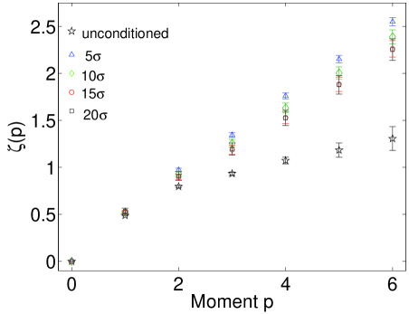
Abbildung 3: Scaling exponents $\zeta(p)$ versus $p$ for the AE index, shown in the same format as figure 2

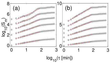
Abbildung 4: Structure functions of the AE index estimated for orders $p=[1,6]$ by method (16) (a) and by method (17) (b).

3 Low Order Moments and Non Uniqueness: Comparison with a fractional Brownian surrogate.

Equation (14) expresses the PDF as an expansion in the moments to all orders. It follows that distinct timeseries can share the first few moments and therefore if scaling, may also share the same Hurst exponent and corresponding exponent of the power law power spectrum. Having estimated the scaling exponent of the AE index as above we can construct a time series with the same second moment from a fractional Brownian motion to illustrate this.

The fractional Brownian walk was generated using the method described in Appendix 3 of [Peters, (1996)]. The algorithm takes a series of Gaussian random numbers and approximates a finite correlation time by weighting past values according to a power law function. In our case 1024 Gaussian samples were used to create each increment of fractional walk. The resulting time series is comprised of $7.5\times 10^{5}$ increments.

Figure 5 shows the two time series, (i) the interval of AE analyzed above, and (ii) the fBm surrogate. The standard deviation versus $\tau$ for the two time series is shown in Figure 6. The power spectrum of AE (the raw, rather than the differenced variable)( c.f. [Tsurutani et al.(1990), Takalo et al.(1993)]), along with the $\sigma(\tau)$ and the structure functions, show a characteristic break on timescales of 1-2 hours. On times shorter than this, we can obtain a scaling collapse of the PDF (see [Hnat et al.(2003a)], also [Hnat et al. (2005)]. Fluctuations on these timescales share the same second moment as the fBm. In Figure 7 we compare the PDF of these fluctuations and we see that these are very distinct; fBm is defined as having Gaussian increments ([Mandelbrot(2002)]) and this is revealed by the PDF whereas the AE increments are non-Gaussian.

This is an illustration of the fact that the scaling in AE over this region is not necessarily due to time correlation, the “Joseph effectfor which Mandelbrot constructed fractional Brownian motion as a model. Indeed AE has almost uncorrelated differences at high frequencies, as indicated by its nearly Brownian $f^{-2}$ power spectrum ([Tsurutani et al.(1990)]). Rather the scaling is synonymous with the heavy tailed PDF (“Noah effect”) for which [Mandelbrot(2002)] earlier introduced a Lévy model in economics.

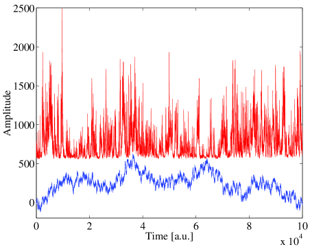
Abbildung 5: A $\sim 1.5$ year interval of AE data (upper trace) is shown alongside a surrogate fBm time series (lower trace) with the same second moment. The traces have been displaced for clarity.

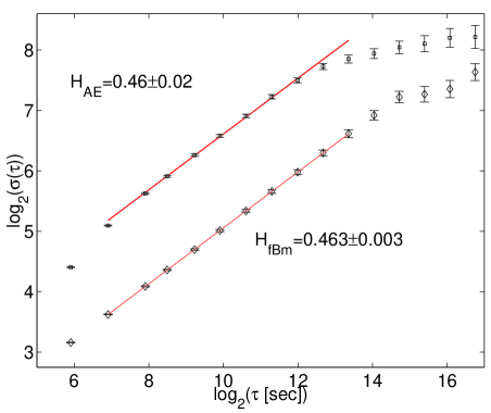
Abbildung 6: Standard deviation of the time series differenced on timescale $\tau$ plotted versus $\tau$ for an interval of AE index data (see text) and an fBm time series constructed with the same second moment. The traces have been displaced for clarity.

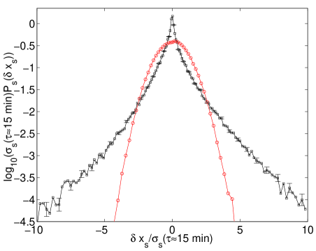
Abbildung 7: PDF of the time series of AE, differenced on timescales less than one hour ($\square$). The PDF of an fBm with the same second moment is shown for comparison ($\circ$).

Finally, we plot in Figure 8 the $\zeta(p)$ versus $p$ obtained from the structure function estimate (17) with $Q=10$ for both time series. We see from the plot that both time series are self affine and to within the uncertainty of the finite length time series, both share values of $\zeta(p)$ for the lowest orders in $p$. However the higher order structure functions reveal the distinct scaling of the two time series.

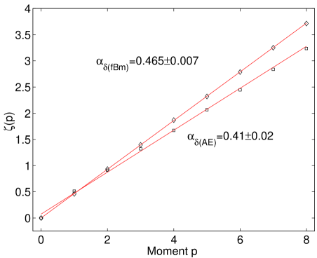
Abbildung 8: Structure functions obtained by conditioning at 10 $\sigma$ for an interval of the AE index, and for a fBm constructed to share the same second moment.

4 Fokker-Planck model

For completeness we now outline how the exponent $\alpha$ of a self affine time series leads to the functional form of $P(y)$ via a Fokker- Planck model of the stochastic process $x(t)$. Here we will consider an approach where scaling is achieved via transport coefficients that are functions of the differenced variable $y(t)$. An alternative approach is via fractional derivatives for the dependent (y) coordinate (see e.g. [Schertzer et al, (2001), Shlesinger et al, (1995)]). These are in principle equivalent (e.g. [Yannacopoulos and Rowlands(1997)]).

We begin with a general form of the Fokker-Planck equation can be written [Gardiner(1986)]:

$$\frac{\partial{P}}{\partial{\tau}}=\nabla_{y}(A(y)P+B(y)\nabla_{y}P),$$ (18)

where $P\equiv P(y,\tau)$ is a PDF for the differenced quantity $y$ that varies with time $\tau$, $A(y)$ is the friction coefficient and $B(y)$ is related to a diffusion coefficient which we allow to vary with $y$. If we now impose the condition that solutions of (18) are invariant under the scaling given by (9), then it is found that both $A(y)$ and $B(y)$ must have the form of power law dependence on $y$. Then as shown in [Hnat et al.(2003b)], (18) takes the form:

$$\frac{\partial{P}}{\partial{\tau}}=\frac{\partial}{\partial{y}}\left[y\mid y\mid^{-1/\alpha}\left(a_{0}P+b_{0}y\frac{\partial{P}}{\partial{y}}\right)\right],$$ (19)

where $a_{0}$ and $b_{0}$ are constants, $\alpha$ is the scaling index derived from the data and $P(y)$, $y$ are unscaled PDF and fluctuations respectively, and where here we have explicitly insisted that the diffusion coefficient $B(y)>0$. Importantly, in a physical system the scaling behaviour (9) is expected to be strongly modified as $y\rightarrow 0$, that is, at the peak of the PDF $P(y)$ since for a sufficiently small difference between two measurements $x(t)$, $y(t,\tau)=x(t+\tau)-x(t)$ will be dominated by the uncertainties in those measurements.

Written in this form equation (19) immediately allows us to identity $B(y)\propto y^{2}\mid y\mid^{-1/\alpha}$ and $A(y)\propto y\mid y\mid^{-1/\alpha}$. Solutions to (19) exist which are functions of $y_{s}=y\tau^{-\alpha}$ only which correspond to stationary solutions with respect to $\tau$. We obtain these by the change of variables ($P,y,\tau\rightarrow P_{s},y_{s}$) of (19):

$$\frac{b_{0}}{a_{0}}y_{s}\frac{dP_{s}}{dy_{s}}+P_{s}+\frac{\alpha}{a_{0}}\mid y_{s}\mid^{\frac{1}{\alpha}}P_{s}=\frac{C\mid y_{s}\mid^{\frac{1}{\alpha}}}{y_{s}}.$$ (20)

This differential equation (20) can be solved analytically with a general solution of the form:

$$P_{s}(y_{s})=\frac{a_{0}}{b_{0}}\frac{C}{|y_{s}|^{a_{0}/b_{0}}}exp\left(-\frac{\alpha^{2}}{b_{0}}\mid y_{s}\mid^{1/\alpha}\right)$$

$$\times\int_{0}^{y_{s}}\frac{\mid y_{s}^{\prime}\mid^{\frac{a_{0}}{b_{0}}}exp\left(\frac{\alpha^{2}}{b_{0}}\mid y_{s}^{\prime}\mid^{1/\alpha}\right)}{\mid y_{s}^{\prime}\mid^{2-\frac{1}{\alpha}}}d(y_{s}^{\prime})+k_{0}H(y_{s}),$$ (21)

where $k_{0}$ is a constant and $H(y_{s})$ is the homogeneous solution:

$$H(\delta x_{s})=\frac{1}{\mid y_{s}\mid^{a_{0}/b_{0}}}exp\left(-\frac{\alpha^{2}}{b_{0}}\mid y_{s}\mid^{1/\alpha}\right).$$ (22)

Power law scaling for arbitrary $y$ leads to singular behaviour of this solution at $y\rightarrow 0$. We do not however expect this to describe a physical system as $y\rightarrow 0$ as discussed above. For (21) to describe a PDF we require that its integral is finite. We can discuss this by considering the behaviour close to the singularity:

$$\lim_{y_{s}\rightarrow 0}P(y_{s})\simeq\frac{a_{0}}{b_{0}}\frac{C}{\mid y_{s}\mid^{\frac{a_{0}}{b_{0}}}}\int^{y_{s}}_{0}\frac{\mid y_{s}^{\prime}\mid^{\frac{a_{0}}{b_{0}}}dy_{s}^{\prime}}{y_{s}^{\prime 2-\frac{1}{\alpha}}}+\frac{k_{0}}{\mid y_{s}\mid^{\frac{a_{0}}{b_{0}}}}=C+\frac{k_{0}}{\mid y_{s}\mid^{\frac{a_{0}}{b_{0}}}}$$ (23)

The integral of (23) is finite for $0\leq a_{0}/b_{0}<1$ and $0<\alpha\leq 1/2$ (a subdiffusive process) so that within this range the integral of (21) will be finite also as required. Outside of this range it can only be considered as an asymptotic solution. However, we can consider the generalization $y\rightarrow y+\epsilon$ in the above, where $\epsilon$ is a constant of magnitude that is small compared to, say, the values of $\sigma(\tau)$ for the physical system under study. This eliminates the singular behaviour and corresponds (for $y$ small) to the addition of low amplitude Gaussian noise as can be seen from the form of the corresponding Langevin equation (24) below. Physically this corresponds to a simple model for the statistical behaviour of the observational uncertainties in the data which may dominate as the differenced quantity $y\rightarrow 0$.

Expression (21) is then a family of solutions for the PDF of self affine time series. This provides a method to test for self affinity that does not directly rely on determining the scaling exponents to high order from the structure functions. Having determined the exponent $\alpha$ from the scaling of a low order moment (say, the standard deviation) one can then perform a scaling collapse on the PDF; this should then also be described by the corresponding solution of (21) (see [Hnat et al.(2003b), Hnat et al. (2005)] for examples).

It is well known that a Fokker Planck equation is simply related to a Langevin equation (see e.g. [Gardiner(1986)]). A nonlinear Langevin equation of the form

$$\frac{dy}{dt}=\beta(y)+\gamma(y)\xi(t),$$ (24)

where $\beta(y)$ is a $y$ -dependent force term and $\gamma(y)$ is a $y$ -dependent noise strength, can be shown ([Hnat et al.(2003b)]) to correspond to (18) and in that sense to describe the time series. In (24) the random variable $\xi(t)$ is assumed to be $\delta$-correlated, i.e.,

$$<\xi(t)\xi(t+\tau)>=\sigma^{2}\delta(\tau).$$ (25)

Consistency with equation (1) is achieved in the data analysis by forming each time series $y(t,\tau)$ with non-overlapping time intervals $\tau$. Defining $D_{0}=<\xi^{2}(t)>/2$ we then obtain:

$$\gamma(y)=\sqrt{\frac{b_{0}}{D_{0}}}y|y|^{-\frac{1}{2\alpha}},$$ (26)

and

$$\beta(y)=\left[b_{0}(1-\frac{1}{2\alpha})-a_{0}\right]y|y|^{-\frac{1}{\alpha}}.$$ (27)

With $\alpha=1/2$ and $a_{0}=0$ one recovers the Brownian random walk with (18) reduced to a diffusion equation with constant diffusion coefficient.

Interestingly, [Beck(2001)] has independently proposed a nonlinear Langevin equation where $\beta$ but not $\gamma$ varies with $y$. This yields leptokurtic PDFs of the Tsallis functional form.

Finally the variable $\tau$ in (18), and $t$ in (24) can be read in two ways: either as the renormalization variable of the stochastic variable $y(t,\tau)$ or the time variable of $x(t)$ since from (1) $\tau=2^{n}\Delta$ and with the choice $N=2^{n}$ we have $x(t)\equiv y^{n}(t,\tau)$, $\tau\equiv t$ ($n,N$ large). Thus (24) can be seen either as a prescription for generating a self- affine timeseries with scaling exponent $\alpha$, or as describing the renormalization flow.

Empirical determination of the scaling properties and exponents of time series $x(t)$ presents a formidable challenge in testing, and developing, a theoretical understanding of turbulence and other out-of-equilibrium phenomena. In this paper we have discussed the special case of self affine time series by treating the differenced variable $y(t,\tau)=x(t+\tau)-x(t)$ as increments of a stochastic process (a generalized random walk). We have highlighted two complementary approaches to the data.

The first of these is PDF rescaling; using a low order moment to determine a scaling exponent and then verifying whether this exponent collapses the PDFs of the differenced variable $y(t,\tau)$ over the full range of $y$ accessible from the data. As a corollary this collapsed PDF should also be well described by the solution of a Fokker-Planck equation which has power law transport coefficients.

The second of these is using structure functions to determine the scaling properties of the higher order moments. In a finite length time series the higher order structure functions can be distorted by isolated, extreme events which are not well represented statistically. Using the example of a finite length Lévy flight, we have demonstrated a method for conditioning the time series that can in principle recover the underlying self affine scaling.

Finally, to highlight how both these methods are complementary in quantifying the scaling properties of the time series a fractional Brownian walk was constructed to share the same second moment as an interval of the differenced AE index time series. The two timeseries were demonstrated to possess very different PDF of the differenced variable, and distinct structure functions.

Both of these approaches could in principle be generalized to multifractal time series (see e.g. [Schertzer et al, (2001)]).