Dynamic positive column in long-gap barrier discharges.

Abstract

A simple analytical model of the barrier discharge in a long gap between opposing plane electrodes is developed. It is shown that the plasma density becomes uniform over large part of the gap in the course of the discharge development, so that one can speak of a formation of a dynamic positive column. The column completely controls the dynamics of the barrier discharge and determines such characteristics as the discharge current, discharge duration, light output, etc. Using the proposed model, all discharge parameters can be easily evaluated.

I INTRODUCTION

Dielectric barrier discharges are typically generated in gas gaps between two electrodes covered with dielectric layers. Sinusoidal or square-wave voltage with frequencies ranging from few kHz to hundreds of kHz are used to generate the discharges. The product of the gas pressure and the distance between the dielectric surfaces $pD$ can vary quite significantly. In the present paper we consider barrier micro-discharges such as used in Plasma Display Panels Meunier et al. (1995) and excimer lamps Eliasson and Kogelschatz (1991) where $pD\approx 5-50$.

The dynamics of a barrier discharge during one pulse of the applied square-wave voltage was considered in detail analytically in our previous work Khudik et al. (2003), where it was shown that at high overvoltage the discharge develops into an ionization wave, whose velocity is determined primarily by the charge production rate in the cathode fall region. This wave moves from the anode toward the cathode, resulting in contraction of the cathode fall region and increase of the electric field within this region. Upon reaching the cathode, the ionization wave can either quickly disappear (when the capacitance of the dielectric layer is small) or transform into a quasi-stationary DC cathode fall (when the capacitance is large). The main assumption of that work was that the resistance of the plasma trail, created by the ionization wave, can be neglected.

In the present paper we consider the opposite case, when the barrier discharge dynamics is strongly influenced by the plasma trail which electrically connects the anode with the cathode fall region. As will be shown below, in the case of a long gap the plasma trail becomes uniform over the large part of the gap, virtually forming a dynamic positive column. The uniformity of the column enables us to consider it simply as a variable resistor through which the cathode fall (CF) charges the dielectric layer capacitor (see Fig. 1). When the capacitance is large, one can introduce further simplifications into the model. In this case the CF is, in essence, quasi-stationary and its V-I characteristics can be approximated by those of the DC cathode fall Yu. P. Raizer (c1991).

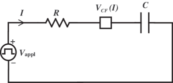
Figure 1: Equivalent circuit of a long-gap barrier discharge.

In our work we neglect the volume and near-wall recombination of charged particles, which if included into consideration would only increase the resistance of the positive column and enhance its role in the barrier discharge dynamics.

Although dynamic characteristics of barrier discharges have been already extensively studied via computer simulations (see Ref. Boeuf (2003) and references therein), it remained unclear, for example, what processes control the duration and amplitude of the current pulse. The proposed model answers this question and can be used to estimate various parameters of long-gap barrier discharges between opposing plane electrodes. This type of discharges (as well as Weber (2001); Schermerhorn et al. (2000); Kawai et al. (2004)) may prove to be a viable alternative to near-surface discharges Punset et al. (1999); Rauf and Kushner (1999); Khudik et al. (2005, ) favored nowadays in Plasma Display Panel industry.

II Qualitative consideration and basic equations

We will consider discharges in a gas gap between opposing plane electrodes covered by dielectric layers of thickness $d$ and dielectric constant $\epsilon$. We assume that the gap length $L_{g}$ is much larger than the length of the normal cathode fall,

$$L_{g}\gg L_{\textrm{norm}}.$$ (1)

It is also assumed that the dielectric layer capacitance is large, i.e. the effective thickness of dielectric layers is small,

$$2d/\epsilon\lesssim L_{\textrm{norm}}.$$ (2)

For example, in the case of 10%-Xe/90%-Ne mixture at pressure 500 Torr and secondary emission coefficients $\gamma_{Ne}=0.5$ and $\gamma_{Xe}=0.005$, the normal cathode fall length $L_{\textrm{norm}}\sim 6.5\mu m$, the gap length under consideration is from several hundred microns to one millimeter, and the effective thickness of dielectric layers is less than or about several microns.

Although discharges in gaps with such a long distance between the anode and cathode can be initiated in several different ways (by, for example, using a set of auxiliary electrodes), we assume that the Townsend breakdown takes place .

Under these assumptions (long gap, large capacitance, Townsend mechanism of the breakdown), the general picture of the discharge dynamics can be described as follows:

1. Upon application of a sufficiently high voltage across the gap ($U_{\textrm{appl}}>U_{\textrm{br}}$, where $U_{\textrm{br}}$ is the breakdown voltage), the Townsend criterion is satisfied and the positive charge starts to build up in the gap. While the amount of total charge is small (and thus the electric field is undisturbed), it grows exponentially with time.

2. At some moment it reaches a critical value ($\sim\epsilon_{0}V_{\textrm{appl}}/L_{g}$) and causes considerable distortion of the electric field. The field vanishes at the anode and from this moment on there coexist two different regions in the gap: the region filled with plasma (plasma trail) where the electric field is relatively small, and the region of the gap adjacent to the cathode where the electric field is strong and the electron density is negligible. With time, the plasma trail expands toward the cathode while the CF region contracts. At this stage, the process of the plasma trail uniformization begins.

3. When the length of the CF region becomes comparable to $L_{\textrm{norm}}$, it transforms into a quasi-stationary DC cathode fall and the discharge current sharply increases and, after reaching its maximum, decreases. The plasma density in the already uniformized plasma trail (positive column) grows while the electric field there falls (see Fig. 2).

Figure 2: Electric field $E$ and electron density $n_{e}$ in the gap at time moments $t_{1}<t_{2}<t_{3}$ when the discharge current is strong: $I(t_{1})=0.5I_{\textrm{max}}$, $I(t_{2})=I_{\textrm{max}}$, and $I(t_{3})=0.5I_{\textrm{max}}$, where $I_{\textrm{max}}$ is the maximum discharge current.

These processes are accompanied by the intensive deposition of power from the external source into the discharge. At the end of this stage, the main portion of the external voltage drops across the dielectric layer capacitor, which leads to quenching of the discharge.

4. In the afterglow, the number of ions and electrons in the gap gradually decreases through the dissociative recombination of electrons and molecular ions. Charged particles are also pulled out of the plasma toward the dielectric surfaces by the residual (and ambipolar) electric fields. Note that although the discharge current is small during the discharge decay, the voltage transferred to the capacitor is about the normal CF voltage $V_{\textrm{norm}}$ (when $2d/\epsilon\ll L_{\textrm{norm}})$.

The key feature of long-gap barrier discharges is that the plasma trail is uniform during the stage three, when the discharge current is strong. The intrinsic mechanism responsible for the uniformization can be qualitatively explained as follows: Due to the plasma quasi-neutrality, which quickly establishes in the Maxwellian time (see Sec. IV), the particle current is constant throughout the plasma trail. Therefore the electric field is higher in regions where plasma density is lower. The higher electric field results in higher ionization rate, which in turn leads to faster growth of the plasma in these regions and, eventually, to a leveling off of the plasma density.

To find the plasma density in the positive column, one can use the continuity equation for electrons

$$\frac{\partial n}{\partial t}-\frac{\partial n\mu_{e}E}{\partial x}=r(E)\,n,$$ (3)

where $n$ is the electron (plasma) density, $\mu_{e}$ is the electron mobility, $E$ is the electric field in the column, and $r(E)$ is the ionization rate. For simplicity, we omitted the diffusion part of the electron flux in Eq. (3). Neglecting the motion of ions (ion mobility is several hundred times lower than the electron mobility) and using the constancy of the particle current, one can immediately arrive at the following relationship between the plasma density and the electric field in the positive column,

$$en\mu_{e}E=I(t)/S,$$ (4)

where $e$ is the elementary charge, $I(t)$ is the discharge current, and $S$ is the cross-sectional area of the discharge. Since the electron mobility is almost constant at small electric fields, from Eq. (4) it follows that

$$\delta nE_{pc}+n_{pc}\delta E=0,$$ (5)

where $\delta n$ and $\delta E$ are perturbations and $n_{pc}$ and $E_{pc}$ are the average values of the plasma density and electric field in the plasma column. Using Eqs. (3)-(5), one can readily obtain

$$\frac{\partial n_{pc}}{\partial t}=r(E_{pc})\,n_{pc},$$ (6)

$$\frac{\partial\delta n}{\partial t}=\Bigg{[}r(E_{pc})-E_{pc}\frac{dr(E_{pc})}{dE_{pc}}\Bigg{]}\;\delta n.$$ (7)

While the obvious equation (6) describes growth of the plasma density in the positive column, Eq. 7 shows fast decay of the density perturbations (since under positive column conditions $E_{pc}r^{\prime}(E_{pc})>r(E_{pc})$). Let us emphasize that, as is seen from our derivation, the mechanism of the positive column uniformization has an entirely dynamic nature and manifests itself regardless of the diffusion processes. It is interesting to note that the uniformization takes place even in a more general case Shvydky et al. (2004a) when the discharge can not be treated as quasi-one-dimensional.

In this paper we give a simple analytic description of only the third stage of the discharge development, when discharge current is strong. During this stage, the positive column occupies almost the entire gap, and as seen from Eq. (6) its resistance $R\approx L_{g}/(en_{pc}\mu_{e}S)$ is governed by

$$\frac{dR}{dt}=-r(E_{pc})\,R,$$ (8)

where

$$E_{pc}=\frac{IR}{L_{g}}.$$ (9)

The quasi-stationarity of the cathode fall allows us to use the V-I characteristic of the corresponding DC cathode fall,

$$V_{CF}=V_{CF}(I).$$ (10)

The applied voltage is distributed between the elements of the circuit in Fig. 1 according to the second Kirchoff law,

$$IR+V_{CF}(I)+\frac{q}{C}=V_{\textrm{appl}},$$ (11)

where $C=\epsilon_{0}\epsilon S/2d$ is the capacitance of the dielectric layer capacitor, and the capacitor charge $q$ changes with time as

$$\frac{dq}{dt}=I.$$ (12)

The equations (8)-(12) form the foundation of our model of barrier discharges with long positive columns and a quasi-stationary cathode fall. They must be complemented with the following initial conditions

$$R(t\rightarrow-\infty)=\infty,$$ (13)

$$q(t\rightarrow-\infty)=0.$$ (14)

Note, that at not very high current densities, the DC CF voltage changes insignificantly (see Fig. 3). The case when the $V_{CF}$ is taken constant and equal to $V_{\textrm{norm}}$ is considered in the next section.

Figure 3: V-I characteristics of the DC cathode fall obtained in the fluid approximation for the gas mixture and secondary emission coefficients mentioned at the beginning of Sec. II. Dotted curve corresponds to the unstable subnormal cathode fall.

III Constant CF voltage approximation

When $V_{CF}=V_{\textrm{norm}}=\textrm{const}$, it is convenient to use $R$ and $E_{pc}$ as independent variables. Replacing the $IR$ with $E_{pc}L_{g}$ and after that taking the time derivative of Eq. (11), one can obtain the equation for the electric field in the positive column,

$$\frac{dE}{dt}=-\frac{E}{R\,C},$$ (15)

where the subscript “pc” is omitted for brevity. Eqs. (8) and (15) must be solved with the following initial conditions

$$R(t\rightarrow-\infty)=\infty,$$ (16)

$$E(t\rightarrow-\infty)=E_{0}\equiv\frac{V_{\textrm{appl}}-V_{CF}}{L_{g}}.$$ (17)

Condition (16) indicates that at the beginning, there is no plasma in the discharge gap, and condition (17) directly follows from condition (14) and the Kirchoff’s law (11).

We would like to point out that, based on what was said in the previous section, Eqs. (8) and (15) do not describe the initial stages of the discharge development, when the positive column is being formed, neither do they describe the final stage, when the discharge quenches and the cathode fall dies.

Now let us turn our attention to the analysis of the system of Eqs. (8) and (15). Dividing left and right parts of equation (8) by the corresponding parts of equation (15) and multiplying both parts by $C$ we obtain

$$\frac{d(RC)}{dE}=\frac{r(E)}{E}\ (RC)^{2}.$$ (18)

Integrating this equation with initial conditions (16) and (17) gives

$$\frac{1}{RC}=\bar{r}(E,E_{0}),$$ (19)

where

$$\bar{r}(E,E_{0})\equiv\int_{E}^{E0}\frac{r(E)}{E}\,dE.$$ (20)

Substitution of (19) into (15) leads to a differential equation for the electric field,

$$\frac{dE}{dt}=-E\;\bar{r}(E,E_{0}),$$ (21)

which should be solved with the initial condition (17). From this equation, one can see that the time evolution of the electric field in the neutral column depends only on its initial value and the ionization rate, and does not depend explicitly on the electron mobility. Because the right part of equation (21) is always negative, the electric field monotonically decreases with time from $E_{0}$ to zero. The discharge current in our model is uniquely determined by the electric field,

$$I\equiv\frac{EL_{g}}{R}=L_{g}CE\;\bar{r}(E,E_{0}).$$ (22)

It goes from zero (at $E=E_{0}$), trough the maximum (at $E=E_{*}$), to zero again (at $E=0$), see Fig. 4.

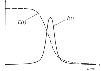
Figure 4: Typical dependence of $I$ and $E$ on time.

The electric field $E_{*}$ at the current maximum can be determined from the extremum condition $dI(E)/dE=0$, which, with the use of Eq. (22), can be written as

$$r(E_{*})=\bar{r}(E_{*},E_{0}).$$ (23)

The typical shape of the function $r(E)/E$ (which is proportional to the the ionization coefficient $\alpha(E)$) as well as the graphical solution of equation (23) is given in Fig. 5.

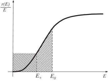
Figure 5: Graphical solution of equation (23). Area of the dashed rectangle on the left is equal to $r(E_{*})$, while the area of the dashed region under the $r(E)/E$ curve on the right is equal to $\bar{r}(E_{*},E_{0})$. These areas are equal when $E_{*}$ is the electric field at the current maximum.

From this figure, one can see, in particular, that always $E_{0}/2<E_{*}<E_{0}$. If $r(E)/E$ grows faster than the linear function, then $E_{0}/\sqrt{3}<E_{*}<E_{0}$.

Using Eqs. (22) and (23), the expression for maximum current can be written as

$$I_{\textrm{max}}=CL_{g}E_{*}\,r(E_{*}).$$ (24)

This equation shows that in the present model the maximum current is proportional to the dielectric layer capacitance. Dependence on the gap length $L_{g}$ is more complicated, since $E_{*}$ also depends on $L_{g}$ (through $E_{0}$).

The time duration $\tau_{\textrm{cur}}$ of the current pulse can be defined as the ratio of transferred charge $Q_{\textrm{tr}}=C\,(V_{\textrm{appl}}-V_{CF})=CL_{g}E_{0}$ to the maximum current,

$$\tau_{\textrm{cur}}\equiv\frac{Q_{\textrm{tr}}}{I_{\textrm{max}}}=\frac{E_{0}}{E_{*}\,r(E_{*})}.$$ (25)

It is useful to note that when $r(E)/E$ grows faster than the linear function, then

$$\tau_{\textrm{cur}}>\frac{3\sqrt{3}}{r(E_{0})}\approx\frac{5.2}{r(E_{0})}.$$ (26)

For a steeper dependence of the ionization coefficient on the electric field, the numerical coefficient in Eq. (26) is even greater.

From (19) immediately follow the expressions for the final resistance of the positive column,

$$R(t=\infty)=\frac{1}{C\,\bar{r}(0,E_{0})},$$ (27)

and for the final plasma density in the column,

$$n(t=\infty)=\frac{C\,L_{g}}{e\mu_{e}S}\,\bar{r}(0,E_{0}).$$ (28)

Using the expression for the ionization coefficient $\alpha=r/\mu_{e}E$, the ratio of the total number of electrons (ions) created in the positive column $N=nL_{g}S$ to the number of transferred electrons (ions) $Q_{\textrm{tr}}/e$ can be written in the form

$$\frac{eN}{Q_{\textrm{tr}}}=\langle\alpha\rangle L_{g},$$ (29)

where

$$\langle\alpha\rangle=\frac{1}{E_{0}}\int_{0}^{E0}\alpha(E)\,dE.$$

Note that $\langle\alpha\rangle<0.5\alpha(E_{0})$ if $\alpha(E)$ grows faster than the linear function. If, in addition to that, $V_{\textrm{appl}}\leq V_{\textrm{br}}+V_{\textrm{norm}}$, then there is a practically useful estimate for the number of charged particles created in the positive column,

$$eN\lesssim\frac{1}{2}\alpha(E_{0})L_{g}Q_{\textrm{tr}}<\frac{1}{2}\ln\big{(}1+\frac{1}{\gamma}\big{)}CV_{\textrm{appl}}.$$ (30)

This expression gives reasonable estimates far beyond the applicability of our model. Note that since the electric field is small in the positive column, in the case of noble gas mixtures, mainly the ions of species with the lower ionization potential are created there.

Similar formulae can be obtained for the number of excited atoms (molecules) created in the positive column during the discharge,

$$\frac{eN_{\textrm{exc}}}{Q_{\textrm{tr}}}=\langle\alpha_{\textrm{exc}}\rangle L_{g},$$ (31)

$$\langle\alpha_{\textrm{exc}}\rangle=\frac{1}{E_{0}}\int_{0}^{E0}\frac{r_{\textrm{exc}}(E)}{\mu_{e}E}\,dE,$$

where $r_{\textrm{exc}}$ is the excitation rate. Again, in the case of noble gas mixtures, mostly the species with lower excitation energies get excited.

Using Eqs. (21) and (22), the energy deposited into the positive column can be estimated as

$$W_{pc}=\frac{1}{2}C(V_{\textrm{appl}}-V_{CF})^{2},$$ (32)

while the total energy which goes from the external source into the discharge is

$$W_{\textrm{tot}}=\frac{1}{2}CV_{\textrm{appl}}^{2}.$$ (33)

Note, that the same amount of energy, $CV_{\textrm{appl}}^{2}/2$, is stored in the capacitor and is recovered during the next discharge pulse.

The difference between Eqs. (33) and (32) gives the amount of energy that goes (in the considered approximation) into the cathode fall,

$$W_{CF}=\frac{1}{2}C\big{[}V_{\textrm{appl}}^{2}-(V_{\textrm{appl}}-V_{CF})^{2}\big{]}.$$ (34)

IV Discussion

To verify the validity of the approximation $V_{CF}=V_{\textrm{norm}}$, one should substitute $I_{\textrm{max}}$ from Eq. (24) into the V-I characteristics of the DC cathode fall (10) and make certain that

$$V_{CF}(I_{\textrm{max}})\approx V_{\textrm{norm}}.$$ (35)

If the obtained CF voltage is noticeably higher than the normal CF voltage, one should analyze the full system of Eqs. (8)-(12), i.e. use the more accurate $V_{CF}=V_{CF}(I)$ approximation instead of the $V=V_{\textrm{norm}}$ approximation.

In Figs. 6-8

Figure 6: Renormalized discharge current for $L_{g}=800\mu m$ and $V_{\textrm{appl}}=390V$: (1) $V_{CF}=V_{\textrm{norm}}$ approximation; (2) fluid simulation for $2d/\epsilon=1\mu m$; (3), (4) fluid simulation and $V_{CF}=V_{CF}(I)$ approximation for $2d/\epsilon=0.1\mu m$; (5) fluid simulation for $2d/\epsilon=10\mu m$. Time is measured from the moment of maximum of the currents.

Figure 7: The same as in Fig. 6 but for $L_{g}=800\mu m$ and $V_{\textrm{appl}}=450V$.

Figure 8: The same as in Fig. 6 but for $L_{g}=400\mu m$ and $V_{\textrm{appl}}=320V$.

are shown results obtained from our model and from fluid simulations under different discharge conditions. A striking feature of all these figures is that the amplitude of the renormalized current $I/C$ changes by only a factor of $2-3$ when the capacitance $C$ changes by two orders of magnitude (compare curves 2,3 and 5). A prediction of our model that $I/C$ does not depend on $C$ (see Eq. (24)) is qualitatively correct even when the criterion (2) of the model applicability is not satisfied. For curve 5, the effective dielectric thickness $2d/\epsilon=10\mu m$ is greater than the normal CF length $L_{\textrm{norm}}\approx 6.5\mu m$, so that the CF is not quasi-stationary but dynamic!

Understandably, the $V_{CF}=V_{\textrm{norm}}$ approximation overestimates the amplitude of the discharge current, since $V_{\textrm{norm}}$ is the minimal voltage on the cathode fall; this overestimation is more pronounced for shorter gaps.

Another interesting feature of the long-gap discharge dynamics is that the duration of the current pulse increases with increase of the gap length (compare Fig. 8 with Figs. 6 and 7), which is not at all obvious since the applied voltage is greater in the case of the longer gap. Qualitatively this discharge property is attributed to the increase in inertia of the positive column with its length.

Note also that in the case of the large capacitance (abnormal quasi-stationary CF, see curve 3), the discharge current grows quickly and falls slowly. In the opposite case of the small capacitance (dynamic CF, see curve 5), the current grows somewhat slower than it falls.

Similar to DC discharges, the positive column in barrier discharges is more efficient source of light (radiation) than the cathode fall. In the positive column, where the electric field is weak, almost all the deposited energy goes into excitation of atoms, while in the cathode fall significant portion of the energy is spent on the ion heating, and, because the electric field is strong, a considerable part of the rest goes into ionization of atoms rather than excitation. It is obvious that the case when the cathode fall is very abnormal (i.e. when the $C$ is very large) is not optimal for the light production. The question of the optimal capacitance of dielectric layers – i.e. the optimal relationship between $2d/\epsilon$ and $L_{\textrm{norm}}$ (which determines to what degree the CF is dynamic) – should be dealt with in the context of concrete discharge parameters.

At the end of this section, let us make several remarks regarding the quasi-neutrality of the plasma in the positive column and possible generalizations of our model. The quasi-neutrality results from the fact that Maxwellian relaxation time is much less than the time of plasma growth in the column (which is of the order of $\tau_{\textrm{cur}}$). Using Eq. (28), one can estimate

$$\tau_{m}=\frac{\epsilon_{0}}{e\mu_{e}n}\sim\frac{\epsilon_{0}S}{CL_{g}\bar{r}(0,E_{0})}=\frac{2d}{\epsilon L_{g}\bar{r}(0,E_{0})}.$$

Since $\bar{r}(0,E_{0})=\bar{r}(0,E_{*})+\bar{r}(E_{*},E_{0})>r(E_{*})\sim\tau_{\textrm{cur}}^{-1}$, the quasi-neutrality condition takes the form

$$\frac{\tau_{m}}{\tau_{\textrm{cur}}}\sim\frac{2d}{\epsilon L_{g}}\ll 1.$$ (36)

Our model allows us to include plasma losses due to ambipolar diffusion to the walls surrounding the discharge volume and due to recombination by subtracting from the r.h.s. of Eq. (6) the terms $\tau^{-1}_{\textrm{dif}}n_{pc}$ ($\tau_{\textrm{dif}}$ is the characteristic ambipolar diffusion time) and $k_{\textrm{r}}n_{pc}^{2}$ ($k_{\textrm{r}}$ is the recombination coefficient). Note, however, that the side walls can strongly influence the breakdown stage of the discharge Shvydky et al. (2004b) and can even lead to the formation of near-dielectric-surface discharge rather than the volume one.

V Conclusion

The dynamics of a barrier discharge between opposing electrodes separated by a long gap which is filled with a mixture of noble gases has been considered. It has been shown that during the discharge development, there forms a region between the anode and the cathode fall similar to a DC positive column, where the plasma density and electric field are uniform but, in contrast to a DC case, change in time. The mechanism of the positive column uniformization has an entirely dynamic nature. It is caused by the ionization processes and has nothing to do with the diffusion.

A simple discharge model allowed us to obtain useful estimates for the plasma density, number of excitations and ionizations, and power consumption; it also helped to capture non-trivial trends in the dependence of the discharge current on discharge parameters.

References

- Meunier et al. (1995) J. Meunier, P. Belenguer, and J. P. Boeuf, J. Appl. Phys. 78, 731 (1995).
- Eliasson and Kogelschatz (1991) B. Eliasson and U. Kogelschatz, IEEE Trans. Plasma Sci. 19, 1063 (1991).
- Khudik et al. (2003) V. N. Khudik, V. P. Nagorny, and A. Shvydky, J. Appl. Phys. 94, 6291 (2003).
- Yu. P. Raizer (c1991) Yu. P. Raizer, Gas Discharge Physics (Berlin ; New York : Springer-Verlag, c1991).
- Boeuf (2003) J. P. Boeuf, J. Phys. D: Appl. Phys. 36, R53 (2003).
- Weber (2001) L. Weber, US Patent 6184848b1 (2001).
- Schermerhorn et al. (2000) J. D. Schermerhorn, E. Anderson, D. Levison, C. Hammon, J. S. Kim, B. Y. Park, J. H. Ryu, A. Shvydky, and A. Sebastian, SID 00 Digest 31, 106 (2000).
- Kawai et al. (2004) S. Kawai, K. Tachibana, J. Oh, H. Asai, N. Kikuchi, and S. Sakamoto, Int. Display Workshop IDW’04 pp. 1059–1062 (2004).
- Punset et al. (1999) C. Punset, S. Cany, and J. P. Boeuf, J. Appl. Phys. 86, 124 (1999).
- Rauf and Kushner (1999) S. Rauf and M. J. Kushner, J. Appl. Phys. 85, 3460 (1999).
- Khudik et al. (2005) V. N. Khudik, V. P. Nagorny, and A. Shvydky, J. SID. 13, 147 (2005).
- (12) V. N. Khudik, A. Shvydky, V. P. Nagorny, and C. E. Theodosiou, to be published in 4th Triennial Special Issue of the IEEE Transactions on Plasma Science ”Images in Plasma Science”, April 2005.
- Shvydky et al. (2004a) A. Shvydky, V. N. Khudik, V. P. Nagorny, and C. E. Theodosiou, Dynamics of the breakdown in a discharge gap at high overvoltages, GEC’57, Sept. 26-29 (2004a).
- Shvydky et al. (2004b) A. Shvydky, V. N. Khudik, and V. P. Nagorny, J. Phys. D: Appl. Phys. 37, 2996 (2004b).