Theoretical Study of Pressure Broadening of Lithium Resonance Lines by Helium Atoms

Abstract

Quantum mechanical calculations are performed of the emission and absorption profiles of the lithium $2s$-$2p$ resonance line under the influence of a helium perturbing gas. We use carefully constructed potential energy surfaces and transition dipole moments to compute the emission and absorption coefficients at temperatures from $200$ to $3000$ K at wavelengths between $500$ nm and $1000$ nm. Contributions from quasi-bound states are included. The resulting red and blue wing profiles are compared with previous theoretical calculations and with an experiment, carried out at a temperature of $670$ K.

I Introduction

It has been argued that prominent features in the spectra of brown dwarfs and extra-solar planets may be attributed to the resonance lines of the alkali metal atoms, broadened by collisions with the ambient hydrogen molecules and helium atoms burrows01 ; seager00 ; brown01 ; allard03 ; burrows03 . The interpretations of the measured profiles which yield information on the temperatures, densities, albedos and composition of the atmospheres are based on models of the line-broadening. Recent studies of the potassium and sodium lines have employed classical and semi-classical scattering theories burrows03 ; nefedov99 ; scheps75 . Jungen and Staemmler jungen88 have obtained detailed emission and absorption profiles (in arbitrary units) for the resonance line of lithium for a wide range of temperatures and Erdman et al. erdman04 have presented measurement of the absorption profile of lithium in a gas of helium at a temperature of $2033$ K together with the results of a quasistatic semiclassical theory.

In this paper, we consider the pressure broadening of the $2p$-$2s$ resonance line of lithium arising from collisions with helium atoms. We carry out full quantitative quantum-mechanical calculations of the emission and absorption coefficients in the red and blue wings. We include contributions from quasi-bound states and we allow for the variation of the transition dipole moment with internuclear distance. We present results for temperatures between 200K and 3000K and we compare with the emission coefficient that has been measured at 670K scheps75 and with calculations of Herman and Sando herman78 at 670K.

II Theory

For a system consisting of a mixture of lithium in a bath of helium atoms, the emission spectrum of the lithium $2p$-$2s$ atomic line has both blue and red wings due to collisions with helium. If the gas densities are low enough that only binary collisions occur, the problem is reduced to the radiation of temporarily formed LiHe molecules. The broadened $2p$-$2s$ atomic emission line corresponds to transitions from the excited A${}^{2}\Pi$ and B${}^{2}\Sigma$ electronic states of the LiHe molecule to the ground X${}^{2}\Sigma$ state. The X${}^{2}\Sigma$ and B${}^{2}\Sigma$ states have no bound states and the A${}^{2}\Pi$ state has a shallow well which supports seven bound ro-vibrational levels. The level $v=6$ is very close to the dissociation limit and it may not be found in practice. In any case it behaves as if it belonged to the continuum. We consider both bound-free and free-free transitions.

The emission coefficient is defined as the number of photons with frequency between $\nu$ and ($\nu+d\nu$) emitted per unit time per unit volume per unit frequency interval, which for bound-free transitions is given by herman78 ; sando71e ; woerd85

$$k_{\nu}^{b-f}(a\rightarrow b)=\omega n_{Li}n_{He}\frac{64\pi^{4}\nu^{3}}{3hc^{3}}\frac{1}{Q_{T}}\frac{2\pi}{\hbar}\cdot\Gamma^{bf}$$ (1)

and for free-free transitions by herman78 ; sando71e ; woerd85

$$k_{\nu}^{f-f}(a\rightarrow b)=\omega n_{Li}n_{He}\frac{64\pi^{4}\nu^{3}}{3hc^{3}}\frac{1}{Q_{T}}\frac{2\pi}{\hbar^{3}}\cdot\Gamma^{ff},$$ (2)

where $\omega$ is the probability that the initial excited electronic state of LiHe is populated by the collision, which is $\frac{2}{3}$ for the A${}^{2}\Pi$ state and $\frac{1}{3}$ for the B${}^{2}\Sigma$ state. In Eqs. (1) and (2), $n_{Li}$ and $n_{He}$ are the number densities of lithium and helium atoms, respectively, $c$ is the speed of light, and $Q_{T}=(2\pi\mu kT/h^{2})^{3/2}$ is the translational partition function for relative motion, $\mu$ is the reduced mass of the collision pair, $k$ is Boltzmann’s constant and $T$ is the temperature. $\Gamma^{bf}$ and $\Gamma^{ff}$ are defined by

$$\Gamma^{bf}=\sum_{v}\sum_{J}g(v,J)|\langle g_{b}^{E_{b},J}|D|g_{a}^{v,J}\rangle|^{2},$$ (3)

and

$$\Gamma^{ff}=\sum_{J}(2J+1)\int dE_{a}\exp(-E_{a}/kT)|\langle g_{b}^{E_{b},J}|D|g_{a}^{E_{a},J}\rangle|^{2},$$ (4)

where $g(v,J)$ is the relative population of levels $(v,J)$ of the A${}^{2}\Pi$ state and $D(R)$ is the electronic transition dipole moment which varies with the nuclear separation $R$. The subscript $a$ denotes the initial state and $b$ the final state. The functions $g^{v,J}$ and $g^{E,J}$ are, respectively, the bound and energy normalized free wave functions determined from the radial Schrödinger equation

$$\frac{d^{2}g(R)}{dR^{2}}+\frac{2\mu}{\hbar^{2}}[E-V(R)-\frac{\hbar^{2}J(J+1)}{2\mu R^{2}}]g(R)=0.$$ (5)

The bound energy $E_{a}^{v,J}$ and free energies $E_{a}$ and $E_{b}$ are measured from the dissociation limit of the excited states and the ground state respectively. The photon frequency $\nu$ is determined by the relation $h\nu=E_{a}-E_{b}+h\nu_{0}$, where $\nu_{0}$ is the atomic line frequency. In writing Eqs. (3) and (4), we may replace the sum of the matrix elements in which $J$ changes by $\pm 1$ by matrix elements in which $J$ does not change.

The sum of Eqs. (1) and (2) is the total photon emission rate. In the limit of high densities, the bound levels of the A${}^{2}\Pi$ state are in thermal equilibrium and $g(v,J)$ is given by

$$g(v,J)=(2J+1)\exp(-E_{a}^{v,J}/kT).$$ (6)

In the limit of low densities, no bound states are populated and only free-free transitions contribute to the emission spectrum.

For absorption, we consider free-bound and free-free transitions from the ground X${}^{2}\Sigma$ electronic state to the excited A${}^{2}\Pi$ and B${}^{2}\Sigma$ states. The absorption coefficient for free-bound transitions is given by doyle68 ; sando71 ; sando73

$$\alpha_{\nu}^{f-b}(b\rightarrow a)=\omega n_{Li}n_{He}\frac{16\pi^{3}\nu}{3hc}\frac{1}{Q_{T}}\frac{\pi}{\hbar}\exp[h(\nu-\nu_{0})/kT]\cdot\Gamma^{bf},$$ (7)

and for free-free transitions by doyle68 ; sando71 ; sando73

$$\alpha_{\nu}^{f-f}(b\rightarrow a)=\omega n_{Li}n_{He}\frac{16\pi^{3}\nu}{3hc}\frac{1}{Q_{T}}\frac{\pi}{\hbar^{3}}\exp[h(\nu-\nu_{0})/kT]\cdot\Gamma^{ff}.$$ (8)

In Eqs. (1), (2), (7) and (8), the emission and absorption coefficients are given in terms of the number of photons in a frequency interval $d\nu$. The photon energies emitted or absorbed are obtained by multiplying $k_{\nu}$ or $\alpha_{\nu}$ by $h\nu$. The coefficients per unit wavelength are obtained by multiplying by $\nu^{2}/c$.

III Potentials and dipole moments

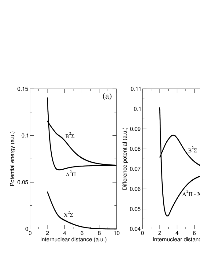
Figure 1: (a) Adopted potentials $V(R)$ in atomic units for the $X^{2}\Sigma$, $A^{2}\Pi$ and $B^{2}\Sigma$ states. (b) Difference potentials $V_{A^{2}\Pi}(R)-V_{X^{2}\Sigma}(R)$ and $V_{B^{2}\Sigma}(R)-V_{X^{2}\Sigma}(R)$ in atomic units.

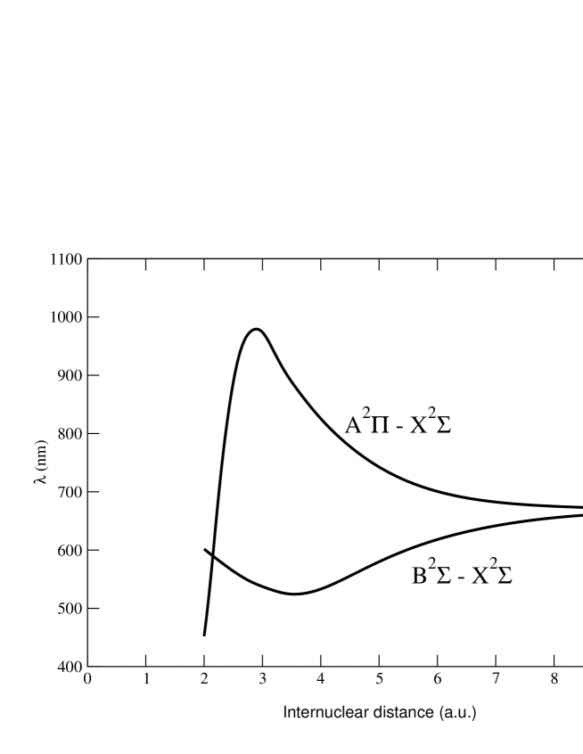
Figure 2: Wavelengths converted from difference potentials for A${}^{2}\Pi$-X${}^{2}\Sigma$ and B${}^{2}\Sigma$-X${}^{2}\Sigma$ transitions.

The potential energy surfaces were constructed to reflect recent calculations. For short and intermediate internuclear distances $R$, the energy points were taken from Ref. czuchaj95 for $3.0\leq R\leq 8.0$, Ref. staemmler97 for $9.0\leq R\leq 19.0$ and Ref. jeung00 for $R=20.0$ for the $X^{2}\Sigma$ state, from Ref. jeung00 for $2.0\leq R\leq 2.75$ and Ref. behmenburg96 for $3.0\leq R\leq 20.0$ for the $A^{2}\Pi$ state, and from Ref. krauss71 for $R=2.0$ and Ref. jeung00 for $3.0\leq R\leq 20.0$ for the $B^{2}\Sigma$ state. At large $R$, the potential energies vary as $-C_{6}/R^{6}$. The theoretical values of $C_{6}$ of $22.51$ for the $X^{2}\Sigma$ state yan96 , $28.27$ for the $A^{2}\Pi$ state yan01 and $50.69$ for the $B^{2}\Sigma$ state yan01 were adopted. For each potential energy curve, the data in different segments were smoothly connected with a cubic spline procedure. The potential energy curves are shown in Fig. 1, along with the difference potentials $V_{A^{2}\Pi}(R)-V_{X^{2}\Sigma}(R)$ and $V_{B^{2}\Sigma}(R)-V_{X^{2}\Sigma}(R)$. In Fig. 2, we present the energy separations as wavelengths $\lambda$ obtained with the classical assumption that the emission occurs through vertical transitions as the particles move along the potential energy curves. The vibrational energy levels of the A${}^{2}\Pi$ state are listed in Table 1. Values of the difference of energy of the $v=0$ and $1$ vibrational levels of the A${}^{2}\Pi$ state have been derived from spectroscopic experiments lee91 . The measured values are $289.9(4)$ cm^-1 and $290.0(3)$ cm^-1, obtained by differencing two A${}^{2}\Pi$–D${}^{2}\Delta$ transitions. From Table 1, we obtain $288.4$ cm^-1. An earlier calculation by Jungen and Staemmler jungen88 yielded $260$ cm^-1.

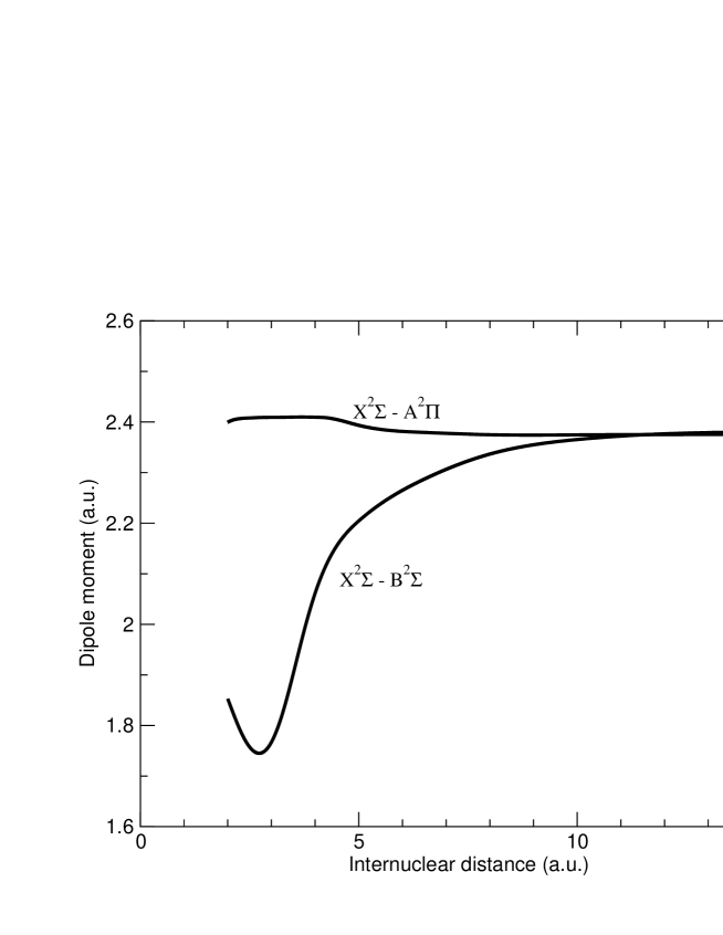
Figure 3: Adopted dipole moment curves for the ${X^{2}\Sigma}-{A^{2}\Pi}$ and ${X^{2}\Sigma}-{B^{2}\Sigma}$ transitions.

The adopted dipole moment curves grycuk are shown in Fig. 3.

IV Calculations

The radial equation (5) was solved using the Numerov method. The integrands of the free-free matrix elements oscillate at large internuclear distances and the integrals fail to converge. They can be transformed by the equation

$$D(R)=\{D(R)-D(\infty)\}+D(\infty).$$ (9)

The matrix element of $\{D(R)-D(\infty)\}$ converges because the operator tends to zero at large $R$. The matrix element of the constant $D(\infty)$ may be written in the formherman78

$$D(\infty)\langle g_{b}^{E_{b},J}|g_{a}^{E_{a},J}\rangle=D(\infty)\langle g_{b}^{E_{b},J}|\Delta V|g_{a}^{E_{a},J}\rangle/(E_{a}-E_{b}),$$ (10)

where $\Delta V=V_{a}(R)-V_{b}(R)$ is the difference potential. The right hand side of (9) is convergent since $\Delta V\rightarrow 0$ for $R\rightarrow\infty$.

The integration over energy in Eq. (4) was carried out using the Gauss-Laguerre method with $100$ points. We also ran the code with $200$ points and found no difference in the results. We included values of $J$ up to $50$ for $T=200$ K and up to $200$ for $T=3000$ K.

Shape resonances occur in scattering by the A${}^{2}\Pi$ potential. They were determined by calculations at high energy resolution. Table 2 is a list of the values of $J$ and the locations and widths $\gamma_{r}^{v,J}$ of the quasi-bound levels. We used Simpson’s rule with energies selected at closely spaced intervals to evaluate the resonance contributions to the energy integrals.

V Results and discussions

The bound-free emission coefficient (1) is a weighted sum of the emission rates of the individual ro-vibrational levels of the A${}^{2}\Pi$ state. The spontaneous transition probabilities are given by

$$W_{\nu}=\frac{64\pi^{4}\nu^{3}}{3hc^{3}}\frac{2\pi}{\hbar}|\langle g_{b}^{E_{b},J}|D|g_{a}^{v,J}\rangle|^{2}.$$ (11)

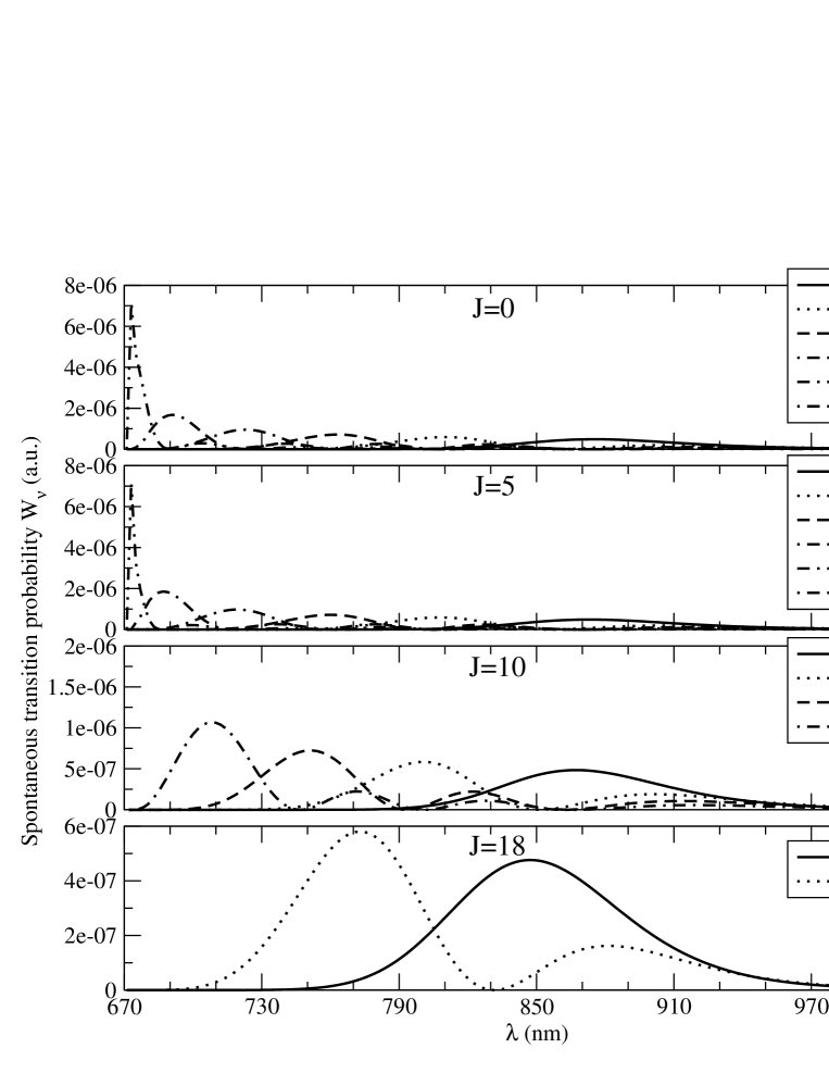
Figure 4: Spontaneous transition probabilities $W_{\nu}$, Eq. (11), in atomic units for vibrational levels $v=0-5$ for $J=0$ (upper panel), $5$ (upper middle panel), $10$ (lower middle panel) and $18$ (lower panel).

In Fig. 4 we plot $W_{\nu}$ in atomic units as a function of wavelength for rotational states $J=0$, $5$, $10$ and $18$ of the vibrational levels $v=0$ to $v=5$. The corresponding lifetimes in seconds are listed in Table 3. For high vibrational levels, they are approaching the limit of the radiative lifetime of the resonance state of the lithium atom which is $27.2$ ns marinescu95 .

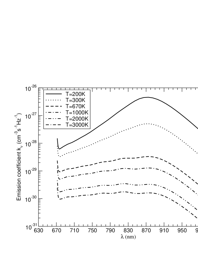
Figure 5: Contributions of bound-free transitions to the total emission coefficients at temperatures $T=200$, $300$, $670$, $1000$, $2000$ and $3000$ K. Unit gas densities are used, $n_{Li}=n_{He}=1$ cm^-3.

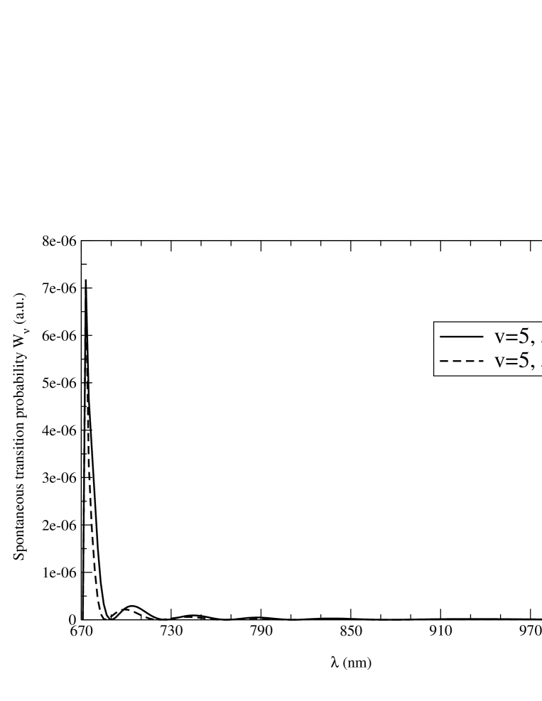
Figure 6: Spontaneous transition probabilities $W_{\nu}$, Eq. (11), in atomic units for ro-vibrational levels $(v,J)=(5,0)$ and $(5,5)$.

In Fig. 5 we present the contributions to the emission coefficient $k_{\nu}$ in units of cm^-3s^-1Hz^-1 of the A${}^{2}\Pi$ state from the bound-free transitions, assuming that the levels are populated in thermal equilibrium at temperatures ranging from $200$ K to $3000$ K. The contributions from the resonances were multiplied by $\gamma_{r}^{v,J}/(\gamma_{r}^{v,J}+\gamma_{i}^{v,J})$, where $\gamma_{r}^{v,J}$ and $\gamma_{i}^{v,J}$ are the resonance and radiative decay widthssando71e , but the effect is negligible. At no temperature and at no frequency is the quasi-bound contribution more than a few percent of the total. The shape of $k_{\nu}$ results from a superposition of the spectra in Fig. 4 weighted by the populations of the ro-vibrational levels. The sharp increase near the resonance wavelength at $670.8$ nm is the contribution from low-lying rotational states of vibrational level $v=5$, illustrated in Fig. 6. A peak in the spectrum at around $870$ nm is apparent at low temperatures but it tends to smooth out at high temperatures. At the higher temperatures, there is a plateau region associated with emission from the attractive region of the potential. The emission decreases rapidly at long wavelengths because there are no values of the internuclear distance $R$ that correspond to wavelengths beyond $1000$ nm, as shown by Fig. 2.

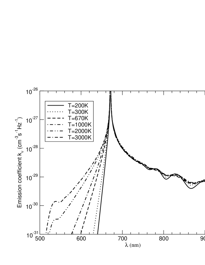
Figure 7: Contributions of free-free transitions to the total emission coefficients at temperatures $T=200$, $300$, $670$, $1000$, $2000$ and $3000$ K. Unit gas densities are used, $n_{Li}=n_{He}=1$ cm^-3.

The calculated free-free photon emission rates $k_{\nu}$ in units of cm^-3s^-1Hz^-1 produced in transitions from the A${}^{2}\Pi$ state to the X${}^{2}\Sigma$ state are presented in Fig. 7. Weak quantum oscillations are found that correspond to transitions from the attractive region of the A${}^{2}\Pi$ potential. There occur rapid increases in $k_{\nu}$ at wavelengths close to the atomic resonance wavelength. At some point as we approach the line center the binary approximation that we have adopted breaks down. Our calculations are valid only in the wings of the line. Studies of the profile at line center have been reviewed by Lewis lewis80 .

The blue wings arise from the B${}^{2}\Sigma$-X${}^{2}\Sigma$ transitions. Only free-free transitions occur and the result is a smooth profile decreasing rapidly with decreasing wavelength except for a weak satellite feature near $536$ nm that is apparent at high temperatures. The behavior is expected from a consideration of Fig. 2 which shows that internuclear distances in the B${}^{2}\Sigma$ state that correspond to short wavelengths are inaccessible. The satellite feature is produced by emission from internuclear distances at which the two potential energy curves are parallel burrows03 . Previous work has located it at $516$ nm krauss71 or $506$ nm scheps75 . There is an indication of the satellite near $530$ nm in an experimental spectrum obtained by Lalos and Hammond lalos62 .

Semi-classical calculations by Jungen and Staemmler jungen88 over a range of temperatures above $200$ K have similar profile shapes to those we obtain with quantum-mechanical calculations. Measurements of the line profile at $670$ K at high pressures have been carried out by Scheps et al. scheps75 and calculations at high and low pressures in the red wing have been made by Herman and Sando herman78 . In Fig. 8 we give a comparison with our results. There is broad agreement between the theoretical low pressure profiles which arise from the free-free transitions. The differences in detail can be ascribed to the adopted interaction potentials. The theoretical calculations of the high pressure profiles have the same shape. They both have a plateau at intermediate wavelengths, increase sharply near the line center and fall off rapidly far in the red wings. They differ quantitatively in the plateau region. Agreement between the present theoretical red and blue wings and experiment is close and it indicates that the binary approximation is valid to within $20$ nm of line center. There may be a discrepancy at wavelengths longer than $950$ nm where the emission coefficient is becoming very small. According to Scheps et al. scheps75 their data at long wavelengths are noisy. The long range interactions should be reliable staemmler97 and we have explored the effects of modifying the X${}^{2}\Sigma$ potential in the short range repulsive region. However we were unable to obtain precise agreement with the measurements.

In Fig. 9, we present the red and blue wings of the line profiles in the high pressure limit for temperatures between $200$ K and $3000$ K. The total energy emitted per second in the red wing at wavelengths longer than $690.8$ nm, given by

$$I_{1}=\int_{0}^{\nu_{0}-\Delta_{1}}h\nu k_{\nu}d\nu,$$ (12)

where $\Delta_{1}$ corresponds to a wavelength shift of $20$ nm red from the line center, and the total energy emitted per second in the blue wing at wavelengths shorter than $650.8$ nm, given by

$$I_{2}=\int_{\nu_{0}+\Delta_{2}}^{\infty}h\nu k_{\nu}d\nu,$$ (13)

where $\Delta_{2}$ corresponds to a wavelength shift of $20$ nm blue from the line center, are listed in Table 4 for temperatures between $200$ K and $3000$ K.

The absorption coefficients are shown in Fig. 10. They are similar in shape to the semi-classical calculations of Jungen and Staemmler jungen88 and of Erdman et al. erdman04 . There is a satellite near $536$ nm which also appears in the emission spectrum but otherwise the absorption coefficients decrease steadily with separation from the position of the resonance line. There is an indication of a satellite near $600$ nm in the calculation of Erdman et al. erdman04 based on different potential curves which may have the same origin.

VI Conclusions

We have carried out quantum mechanical calculations for the Li-He emission and absorption spectra at temperatures from $200$ K to $3000$ K and wavelengths from $500$ nm to $1000$ nm. We find a blue satellite near $536$ nm for $T=3000$ K and a red satellite near $870$ nm for $T\approx 200$–$300$ K in the emission spectra, and a blue satellite near $536$ nm for $T\approx 2000$–$3000$ K in the absorption spectra. At $670$ K, our emission coefficients are in good agreement with experiment.

Table 1: Vibrational energy levels of the A${}^{2}\Pi$ state of the LiHe molecule.

$v$	0	1	2	3	4	5	6
$E^{v,J=0}$ (cm-1)	$-837.7$	$-549.3$	$-327.7$	$-168.2$	$-67.11$	$-15.69$	$-0.9170$

Table 2: Resonance energies $E_{r}^{v,J}$ and widths $\gamma_{r}^{v,J}$ of the quasi-bound levels of the A${}^{2}\Pi$ state.

$J$	$v$	$E_{r}^{v,J}$ (Hartree)	$\gamma_{r}^{v,J}$ (Hartree)
2	1	2.14$\times$10-7	2.1$\times$10-8
6	1	1.34$\times$10-5	6.5$\times$10-7
9	1	1.04$\times$10-5	7.1$\times$10-13
10	1	6.56$\times$10-5	1.2$\times$10-6
11	1	1.19$\times$10-4	1.8$\times$10-5
13	1	9.15$\times$10-5	2.3$\times$10-9
14	1	1.94$\times$10-4	2.1$\times$10-6
15	1	2.91$\times$10-4	2.4$\times$10-5
16	1	1.23$\times$10-4	1.3$\times$10-12
17	1	2.90$\times$10-4	7.0$\times$10-8
18	1	4.50$\times$10-4	6.0$\times$10-6
19	1	1.82$\times$10-4	3.6$\times$10-15
20	1	4.21$\times$10-4	1.6$\times$10-9
21	1	6.57$\times$10-4	7.0$\times$10-7
22	1	2.84$\times$10-4	6.2$\times$10-17
22	2	8.81$\times$10-4	1.7$\times$10-5
23	1	6.07$\times$10-4	3.4$\times$10-11
24	1	9.31$\times$10-4	4.2$\times$10-8
25	1	1.25$\times$10-3	3.0$\times$10-6
26	1	1.55$\times$10-3	3.1$\times$10-5

Table 3: Lifetimes (ns) of selected ro-vibrational levels $(v,J)$ of the A${}^{2}\Pi$ state.

	$v=0$	$v=1$	$v=2$	$v=3$	$v=4$	$v=5$
$J=0$	59.2	51.5	44.1	37.7	32.4	28.6
$J=5$	58.8	50.9	43.5	37.0	31.7	27.7
$J=10$	57.4	49.4	41.8	35.0
$J=18$	53.0	43.7

Table 4: Total energy emitted per second (ergs cm^-3 s^-1) defined in Eqs. (12) and (13) for the red and blue wings, respectively.

T(K)	Red wing	Blue wing
200	4.68$\times$10-25	1.46$\times$10-29
300	7.59$\times$10-26	9.79$\times$10-29
670	1.64$\times$10-26	8.27$\times$10-28
1000	1.22$\times$10-26	1.59$\times$10-27
2000	9.39$\times$10-27	3.51$\times$10-27
3000	8.67$\times$10-27	4.88$\times$10-27

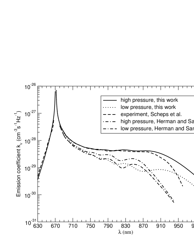
Figure 8: Comparisons of our calculated emission coefficients with experimental measurement of Scheps et al. scheps75 and previous theoretical calculations of Herman and Sando herman78 . For the blue wing, the high and low pressure curves are identical. Unit gas densities are used, $n_{Li}=n_{He}=1$ cm^-3.

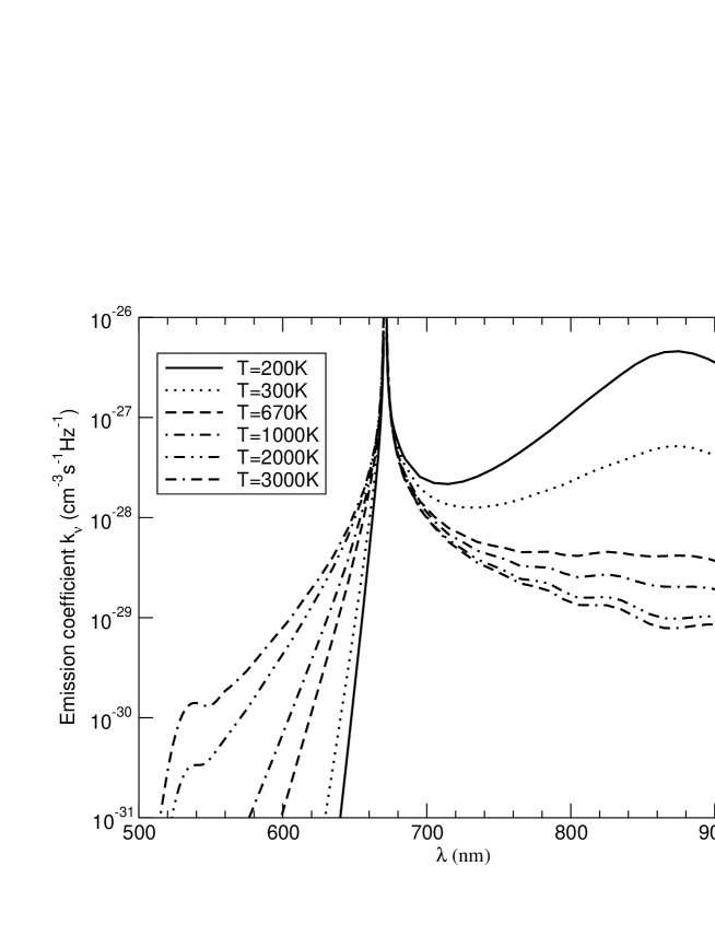
Figure 9: High pressure emission coefficients at temperatures $T=200$, $300$, $670$, $1000$, $2000$ and $3000$ K. Unit gas densities are used, $n_{Li}=n_{He}=1$ cm^-3.

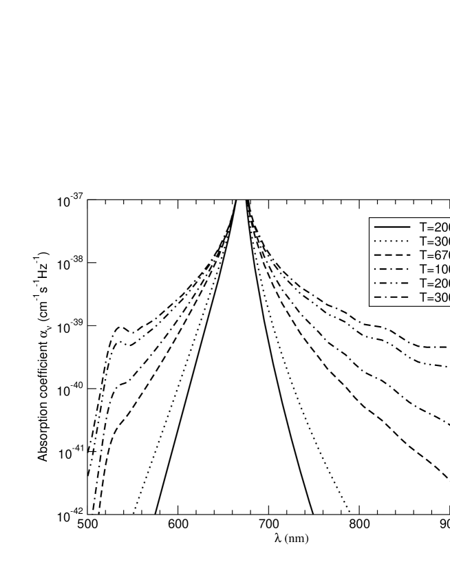
Figure 10: Absorption coefficients at temperatures $T=200$, $300$, $670$, $1000$, $2000$ and $3000$ K. Unit gas densities are used, $n_{Li}=n_{He}=1$ cm^-3.