Application of noise level estimation for portfolio optimization

Abstract

Time changes of noise level at Warsaw Stock Market are analyzed using a recently developed method basing on properties of the coarse grained entropy. The condition of the minimal noise level is used to build an efficient portfolio. Our noise level approach seems to be a much better tool for risk estimations than standard volatility parameters. Implementation of a corresponding threshold investment strategy gives positive returns for historical data.

pacs 05.45.Tp,89.65.Gh

keywords: Noise level estimation, stock market data, time series, portfolio diversification

1 Introduction

Although it is a common believe that the stock market behaviour is driven by stochastic processes voit ; Buchound ; Mantegna it is difficult to separate stochastic and deterministic components of market dynamics. In fact the deterministic fraction follows usually from nonlinear effects and can possess a non-periodic or even chaotic characteristics Peters ; Holyst . The aim of this paper is to study the level of stochasticity in time series coming from stock market. We will show that our noise level analysis can be useful for portfolio optimization.

We employ here a method of noise-level estimation that has been described in details in urbanowicz . The method is quite universal and it is valid even for high noise levels. The method makes use of a functional dependence of coarse-grained correlation entropy $K_{2}(\varepsilon)$ kantzschreiber on the threshold parameter $\varepsilon$. Since the function $K_{2}(\varepsilon)$ depends in a characteristic way on the noise standard deviation $\sigma$ thus $\sigma$ can be found from a shape of $K_{2}(\varepsilon)$. The validity of our method has been verified by applying it for the noise level estimation in several chaotic models kantzschreiber and for the Chua electronic circuit contaminated by noise. The method distinguishes a noise appearing due to the presence of a stochastic process from a non-periodic deterministic behaviour (including the deterministic chaos). Analytic calculations justifying our method have been developed for the gaussian noise added to the observed deterministic variable. It has been also checked by numerical experiments that the method works properly for a uniform noise distribution and at least for some models with a dynamical noise corresponding to the Langevine equation urbanowicz . The method has been already successfully applied for noise level calculations of engine process urbengine and has given similar results to an approach basing on neighboring distances in Takens space urbtakens .

2 Choosing low noise portfolio

In the present paper we define the noise level as the ratio of standard deviation of estimated noise $\sigma$ to the standard deviation of data $\sigma_{data}$

$$NTS=\frac{\sigma}{\sigma_{data}}$$ (1)

In the first step we construct a portfolio from $M$ stocks with the minimal value of the stochastic variable urbAPFA4 . We assume that one can do this by maximization of the following quantity:

$$\mathcal{B}=\sum\limits_{i=1}^{M}\sum\limits_{j=1}^{M}p_{i}p_{j}\frac{\sigma_{i,D}}{\sigma_{i}}\frac{\sigma_{j,D}}{\sigma_{j}}\rho_{i,j}=max$$ (2)

where $\sigma_{i,D}$ is the standard deviation of deterministic part of the stock $i$, $\sigma_{i}$ is the standard deviation of the noise for this stock and $\rho_{i,j}$ is the correlation coefficient between deterministic parts of stocks $i$ and $j$. The maximal value of $\mathcal{B}$ can be received with the help of the steepest descent method by changing variables $p_{i}$ and keeping the normalization constraint $\sum_{i=1}^{M}p_{i}=1$.

In some cases for practical reasons it is more efficient not to minimize the noise level in the portfolio but to maximize it. This is because the method for noise level estimation can fail and it can occasionally give wrong values of $NTS$. When we minimize the noise level it can happen that one stock with an artificially very low noise level dominates the whole portfolio and the risk increases without any additional profit.

3 Investment method

In our investment method we make use of additional information, available due to the knowledge of the noise level, to increase profits from selected portfolios. The simplest approach is to introduce a threshold for a noise level. We divide all portfolios into two classes: profitable and nonprofitable taking into account high or low values of the noise level and a positive or a negative past trend. The partition into high/low noise classes is based on the threshold parameter $NTS_{th}$ that should be optimized. Additionally we label portfolio by calculations of an average return for the last $N_{win}$ data. We use the following algorithm: if the past trend from $N_{win}$ data of the portfolio is positive $m_{p}>0$ and the noise level of the portfolio is small ($NTS_{p}<NTS_{th}$) we consider the portfolio as a profitable. We have a profitable portfolio also when it is more stochastic ($NTS_{p}>NTS_{th}$) but its trend is negative $m_{p}<0$. In the remaining two cases we consider the portfolio as a nonprofitable. In such a way we create the basic strategy giving $\{p_{i}\}$, which involves the information on the noise level and the past trend in the portfolio selection. This basic strategy should then be adjusted using a risk parameter $\mathbf{r}$ that is introduced below. The process of the final portfolio selection is based on the comparison of the optimized portfolio to the simplest portfolio consisting of equal contributions from all stocks ($p_{i}=1/M$, $i=1,...,M$). We set up a composition of the final portfolio $\{\tilde{p}_{i}\}$ with a use of certain risk parameter $\mathbf{r}$ on the preliminary optimized portfolio $\{p_{i}\}$ as follows:

$$\tilde{p}_{i}=\frac{1}{M}+\mathbf{r}\left(p_{i}-\frac{1}{M}\right)$$ (3)

One should mention that for a negative value of the parameter $\mathbf{r}$ we have the opposite investing to the composition $p_{i}$.

At Fig. 2 the level of success of our investment method as a function of the parameter $NTS_{th}$ is shown. Here the percent of success corresponds to a fraction of positive returns from our strategy. We have used a negative risk parameter $\mathbf{r}=-10$ to get a positive profit for small values of $NTS_{th}$: $NTS_{th}<0.85$ in the above simulations. A similar dependence on the parameter $N_{win}$ is shown at Fig. 2. The percent of the success in both cases is above $50\%$ and for some regions of selected parameters the strategy brings positive returns after commissions deduction.

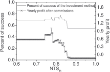
Figure 1: Plot of the investment success as a function of parameter $NTS_{th}$ in the period of January - July 2003 at the Warsaw Stock Exchange ($N_{win}=2500$). Portfolio consists of 18 stocks from WSE.

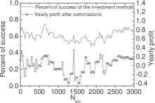
Figure 2: Plot of the investment success as a function of parameter $N_{win}$ in the period of January - July 2003 at Warsaw Stock Exchange ($NTS_{th}=0.85$). Portfolio consists of 18 stocks from WSE.

It is clear that to use our approach we have to find optimal threshold parameters $NTS_{th}$ and $N_{win}$. Our optimization method is quite straightforward and it resembles a genetic algorithm. During the optimization process we change the selection probability for actual values of optimized parameters i.e. we increase the probability if the profit from portfolio is positive and we decrease in the opposite case. The optimization process is terminated when we reach a satisfactory mean value of a yearly profit from past data (here it is $30\%$). In such a way we optimize simultaneously two parameters $N_{win}$ and $NTS_{th}$.

We begin our algorithm by generating randomly chosen stocks in the initial portfolio. Then we randomly select a starting moment for our virtual investment. The next step is to optimize the parameters $N_{win}$ and $NTS_{th}$ using available data from the period prior to the selected starting point. Finally we invest in the portfolio described by the risk value $\mathbf{r}=-3$ (see Eq. 3). The procedure was repeated $10000$ times and at the end we calculated an average profit i.e. the efficiency of the method. At Fig. 4 we show a distribution of returns for our portfolio at Warsaw Stock Exchange. We have calculated recommendations for windows $17-41$ days long on the period July 2002 - December 2003 (see Fig. 4). The annual return received in such a way after commissions substracting is around $56\%$ (the commission level has been set to $0.25\%$). To omit artificially large price changes that can be caused by such effects as stock splitting, extreme returns larger than $12$ standard deviation of data have been rejected.

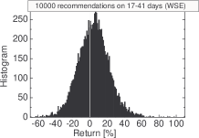
Figure 3: Histogram of returns received by our strategy. The mean return equals to $4.33\%$ while the histogram dispersion is about $17\%$.

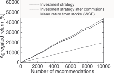
Figure 4: The aggregated return for our investment strategy applied for the Warsaw Stock Exchange. The return corresponds to the mean annual return $56\%$ while the mean annual return of Warsaw Stock Index was about $28\%$ at the same time period.

4 Conclusions

In conclusion we have analyzed noise level for data from Warsaw Stock Exchange. We show that our noise level estimations can be useful for portfolio optimization. The resulting investment strategy brings larger profits than a simple average from the same stocks.

References

- (1) Voit J (2001) The Statistical Mechanics of Financial Markets. Springer-Verlag, Berlin Heidelberg New York Barcelona Hong Kong London Milan Paris Singapore Tokyo
- (2) Bouchaud JP, Potters M (2000) Theory of financial risks - from statistical physics to risk management. Cambridge University Press, Cambridge
- (3) Mantegna RN, Stanley HE (2000) An Introduction to Econophysics. Correlations and Complexity in Finance. Cambridge University Press, Cambridge
- (4) Peters EE (1997) Chaos and Order in the Capital Markets. A new view of cycle, Price, and Market Volatility. John Wiley Sons, New York.
- (5) Hołyst JA et al. (2001) Observations of deterministic chaos in financial time series by recurrence plots, can one control chaotic economy? European Physical Journal B 20:531-535
- (6) Urbanowicz K, Hołyst JA (2003) Noise-level estimation of time series using coarse-grained entropy. Phys. Rev. E 67:046218; http://www.chaosandnoise.org
- (7) Kantz H, Schreiber T (1997) Nonlinear Time Series Analysis. Cambridge University Press, Cambridge
- (8) Kaminski T et al. (2004) Combustion process in a spark ignition engine: Dynamics and noise level estimation. Chaos 14(2):461-466; Litak G et al. (2005) Estimation of a Noise Level Using Coarse-Grained Entropy of Experimental Time Series of Internal Pressure in a Combustion Engine. Chaos Solitons & fractals 23(5):1695-1701
- (9) Urbanowicz K, Hołyst JA (2004) Noise estimation by the use of neighboring distance in Takens space and its application to the stock market data. Proceedings of the Conference Complexity in science and society, International Journal of Bifurcation and Chaos, arXiv:cond-mat/0412098; http://www.chaosandnoise.org
- (10) Urbanowicz K and Hołyst JA (2004) Investment strategy due to the minimization of the noise level in a portfolio. Physica A 344:284-288