Invariant imbedding theory of mode conversion in inhomogeneous plasmas: I. Exact calculation of the mode conversion coefficient in cold, unmagnetized plasmas

Abstract

This is the first of a series of papers devoted to the development of the invariant imbedding theory of mode conversion in inhomogeneous plasmas. A new version of the invariant imbedding theory of wave propagation in inhomogeneous media allows one to solve a wide variety of coupled wave equations exactly and efficiently, even in the cases where the material parameters change discontinuously at the boundaries and inside the inhomogeneous medium. In this paper, the invariant imbedding method is applied to the mode conversion of the simplest kind, that is the conversion of $p$-polarized electromagnetic waves into electrostatic modes in cold, unmagnetized plasmas. The mode conversion coefficient and the field distribution are calculated exactly for linear and parabolic plasma density profiles and compared quantitatively with previous results.

I Introduction

The conversion of one type of wave mode into another type of mode at resonance points in inhomogeneous plasmas and the associated irreversible transfer of wave energy to the mode conversion region are important and extensively-studied phenomena in both space and laboratory plasmas.budden ; ginz ; swanson ; stix ; mjol There exists a vast literature on a large number of mode conversion phenomena involving many different wave modes, which we will not attempt to review here.stix2 ; moore ; chen ; woo ; cairns ; ram ; bellan ; yin ; johnson0 ; johnson1 ; wiles ; lee ; lee2 ; denisov ; piliya ; sc ; pert ; means ; fors ; hink1 ; hink0 ; hink2 ; hink3 Since mode conversion is associated with the singularity of wave functions, theoretical studies encounter great difficulties and often adopt some kind of approximate methods such as the WKB method. In complicated cases where plasma waves are strongly coupled, these approximate methods are often unable to produce sufficiently accurate results. Therefore development of a theoretical method that allows exact solutions to mode conversion problems will be of great value in the study of inhomogeneous plasmas.

In this paper and a series of companion papers to be published later, we will develop an exact theory of mode conversion based on a new version of the invariant imbedding method (IIM) for wave propagation in arbitrarily-inhomogeneous stratified media. The main idea of the IIM is to transform the original boundary value problem of wave equations, which are second-order differential equations, to an initial value problem of coupled first-order ordinary differential equations for the reflection and transmission coefficients and the field amplitudes.bell ; kly0 ; kly1 ; rammal ; kim1 ; kim2 ; kim3 These equations are called the invariant imbedding equations and the independent variable, which is usually the thickness of inhomogeneous media, is called the imbedding parameter. This transformation makes the numerical solution of wave equations much easier.

Our IIM utilizes a rigorous integral representation of wave equations and differs substantially from the better-known IIM presented in Ref. 29.lee ; lee2 ; kim1 ; kim2 ; kim3 More specifically, our method gives the invariant imbedding equations with nonsingular coefficients even in the cases where the material parameters change discontinuously at some discrete points inside the inhomogeneous medium, unlike the imbedding equations derived in Ref. 29. When the inhomogeneity is one-dimensional, which is the case in stratified media, our method can be used to obtain exact solutions for the reflection and transmission coefficients and the electric and magnetic field amplitudes inside arbitrarily-inhomogeneous media. When the inhomogeneity is random, it can be used to obtain the exact disorder-averaged reflection and transmission coefficients and field amplitudes.kim1 Our method can also be used to study the propagation of several coupled waves in both linear and nonlinear media in an exact manner.kim3

In this paper, we apply our IIM to the mode conversion of the simplest kind, that is the conversion and resonant absorption of obliquely-incident $p$-polarized electromagnetic waves into electrostatic modes in cold, unmagnetized plasmas.denisov ; piliya ; sc ; pert ; means ; fors ; hink1 ; hink0 ; hink2 ; hink3 When a $p$ wave of frequency $\omega$ enters a stratified plasma with a monotonically-increasing density profile at an incident angle $\theta$, it propagates first to the cutoff point where the local plasma frequency $\omega_{p}$ equals $\omega\cos\theta$ and is partially reflected. Some fraction of the wave then tunnels to the mode conversion point where $\omega_{p}$ is equal to $\omega$ and is converted to electrostatic modes. Since the generation of electrostatic modes requires the electric field component in the direction of inhomogeneity, only obliquely-incident $p$ waves can produce mode conversion in unmagnetized plasmas.

Mode conversion in unmagnetized plasmas has been studied extensively over many decades and a detailed review of the literature can be found in Ref. 25. In this paper, we restrict our attention to cold plasmas with zero temperature and postpone the discussion of finite temperature effects to future publications. Though our method can be applied to stratified plasmas with arbitrary density profiles very easily, we consider only the cases with linear and parabolic density profiles in this paper. One of the main reasons why we revisit this well-studied problem is to establish the accuracy and efficiency of our method before applying it to more complicated mode conversion problems.

Among a large number of references on the mode conversion in unmagnetized plasmas with a linear density profile in half- or entire space, we mention just two papers. The readers may refer to Ref. 25 for a more complete list of references. Forslund et al. performed a numerical simulation of warm, unmagnetized plasmas at low temperatures.fors The mode conversion coefficient and the field distribution at the lowest temperature they have studied are generally considered to be an accurate solution of the mode conversion problem in cold, unmagnetized plasmas.

Hinkel-Lipsker et al. derived analytical formulas for the mode conversion coefficient in the cases where the density profile is linear and parabolic in entire space.hink1 ; hink0 ; hink2 ; hink3 Their result in the linear case agrees pretty well with Forslund et al.’s result, but there is some numerical discrepancy.hink1 In the parabolic case, they considered the case where the wave frequency is fixed at the value of the local plasma frequency at the peak of the parabolic density profile separately from more general cases where the wave frequency is lower than the peak plasma frequency.hink0 ; hink2 ; hink3

We calculate the mode conversion coefficient and the magnetic field distribution for precisely the same models as those considered in Refs. 24$-$28. We find a very good agreement with the result of Ref. 24 in the linear case, though we believe that the numerical accuracy of our result is better. In the parabolic case, we find substantial differences between our results and those of Refs. 26$-$28. To the best of our knowledge, the results presented in this paper represent the first exact solution of the mode conversion problem in cold, unmagnetized plasmas with linear and parabolic density profiles.

In Sec. II, we introduce the wave equation and the plasma density profiles. In Sec. III, we present the IIM and the invariant imbedding equations for the reflection and transmission coefficients and the field amplitudes. In Secs. IV and V, the results on the case with a linear density profile in entire or half- space are presented. In Sec. VI, the results on the case with a parabolic density profile in entire space are presented. We conclude the paper in Sec. VII.

II Model

We consider a plane, monochromatic and linearly-polarized electromagnetic wave of frequency $\omega$ and vacuum wave number $k_{0}=\omega/c$, incident from a homogeneous region on a stratified inhomogeneous plasma, where the electron density $n$ and the dielectric permittivity $\epsilon$ varies only in one direction in space. We take this direction as the $z$ axis and assume that the inhomogeneous plasma lies in $0\leq z\leq L$ and the wave propagates in the $xz$ plane. Since the plasma is uniform in the $x$ direction, the $x$ component of the wave vector, $q$, is a constant and the dependence on $x$ is taken as being through a factor $e^{iqx}$. When $q$ is nonzero, the wave is said to pass through the plasma obliquely.

For $q\neq 0$, we need to distinguish two independent cases of polarization. In the first case, the electric field vector is perpendicular to the $xz$ plane and the magnetic field vector lies in that plane. This type of wave is known as an $s$ (or TE) wave. In the second case, the magnetic field vector is perpendicular to the $xz$ plane and the electric field vector lies in that plane. Then the complex amplitude of the magnetic field, $B=B(z)$, satisfies

$${{{d^{2}}B}\over{dz^{2}}}-{1\over\epsilon(z)}{{d\epsilon}\over{dz}}{{dB}\over{dz}}+\left[{{k_{0}}^{2}}\epsilon(z)-q^{2}\right]B=0.$$ (1)

This type of wave is called $p$ (or TM) wave. In Eq. (1), we have assumed that the magnetic permeability of the plasma is equal to 1. It is well-known that if the incident wave is $s$-polarized, mode conversion does not occur in unmagnetized plasmas. In this paper, we will consider only the $p$ wave case.

It is straightforward to derive an analytical expression for $\epsilon$ in a cold, unmagnetized electron plasma:

$$\epsilon(z)=1-\frac{{\omega_{p}}^{2}}{\omega\left(\omega+i\gamma\right)},~{}~{}{\omega_{p}}^{2}=\frac{4\pi e^{2}}{m}n(z),$$ (2)

where $\gamma$ is the collision frequency and $\omega_{p}$ is the electron plasma frequency. $e$ and $m$ are the electron charge and mass, respectively. We assume that the wave is incident from region I where $z>L$ and transmitted to region II where $z<0$. The dielectric permittivity is equal to $\epsilon_{1}$ in region I and $\epsilon_{2}$ in region II. The phenomenological collision frequency $\gamma$ is assumed to be zero in regions I and II.

Our method can be applied to the general case where the electron density $n$ is an arbitrary function of $z$. In this paper, we restrict our consideration to three special cases. In Model A, the density depends on $z$ linearly in entire space. In order to treat this case, we assume that the density $n(z)$ is given by

$$n_{A}(z)=n_{0}\left(1-\frac{z-\frac{L}{2}}{\Lambda}\right)$$ (3)

for $0\leq z\leq L$ and take the $L\rightarrow\infty$ limit numerically. The constant $\Lambda$ is the scale length for the linear density profile. We point out that for $z>\Lambda+L/2$, the density takes unphysical negative values. When $L\rightarrow\infty$, $n_{A}(z)$ varies from $-\infty$ at $z=L$ to $+\infty$ at $z=0$. We make a further simplification by assuming that the frequency is fixed at the value of the local plasma frequency at $z=L/2$, which is $\left(4\pi n_{0}e^{2}/m\right)^{1/2}$, and $\gamma\ll\omega$. We make these inessential assumptions just to make our model look exactly the same as the corresponding model in Ref. 25. Then the dielectric permittivity takes the form

$$\epsilon_{A}(z)=\left\{\begin{array}[]{ll}\frac{1}{2}\frac{L}{\Lambda}&~{}~{}\mbox{if $z>L$}\\ \frac{z-\frac{L}{2}}{\Lambda}+i\eta&~{}~{}\mbox{if $0\leq z\leq L$}\\ -\frac{1}{2}\frac{L}{\Lambda}&~{}~{}\mbox{if $z<0$}\end{array}\right.,$$ (4)

where the dimensionless damping parameter $\eta$ is proportional to $\gamma$ and will be sent to zero numerically. We note that in the absence of damping, the dielectric permittivity vanishes at $z=L/2$, where the mode conversion takes place.

In Model B, we assume that the wave is incident from a vacuum on an inhomogeneous plasma, where the electron density depends on $z$ linearly in half-space. The density is given by

$$n_{B}(z)=n_{0}\frac{L-z}{\Lambda}$$ (5)

for $0\leq z\leq L$. In the $L\rightarrow\infty$ limit, $n_{B}(z)$ varies from $0$ at $z=L$ to $+\infty$ at $z=0$. Similarly to the Model A case, we make an assumption that the frequency is fixed at the value of the local plasma frequency at $z=L-\Lambda$, $\left(4\pi n_{0}e^{2}/m\right)^{1/2}$, and $\gamma\ll\omega$. Then the dielectric permittivity has the form

$$\epsilon_{B}(z)=\left\{\begin{array}[]{ll}1&~{}~{}\mbox{if $z>L$}\\ 1+\frac{z-L}{\Lambda}+i\eta&~{}~{}\mbox{if $0\leq z\leq L$}\\ 1-\frac{L}{\Lambda}&~{}~{}\mbox{if $z<0$}\end{array}\right..$$ (6)

The mode conversion occurs at $z=L-\Lambda$ in this case.

In Model C, we assume that the density depends on $z$ parabolically in entire space and is given by

$$n_{C}(z)=n_{0}\left[1-\left(\frac{z-\frac{L}{2}}{\Lambda}\right)^{2}\right]$$ (7)

for $0\leq z\leq L$ and the $L\rightarrow\infty$ limit will be taken numerically. $n_{0}$ is the electron density at the top of the parabolic density profile and $\Lambda$ is the scale length. Assuming that $\gamma\ll\omega$, the dielectric permittivity is given by

$$\epsilon_{C}(z)=\left\{\begin{array}[]{ll}\left(\frac{1}{2}\frac{L}{\Lambda}\right)^{2}&~{}~{}\mbox{if $z>L$}\\ \left(\delta+1\right)\left(\frac{z-\frac{L}{2}}{\Lambda}\right)^{2}-\delta+i\eta&~{}~{}\mbox{if $0\leq z\leq L$}\\ \left(\frac{1}{2}\frac{L}{\Lambda}\right)^{2}&~{}~{}\mbox{if $z<0$}\end{array}\right.,$$ (8)

where $\delta=4\pi n_{0}e^{2}/(m\omega^{2})-1$. If the frequency is fixed at the value of the plasma frequency at the top of the density profile, $\delta$ is equal to zero. When the wave frequency is shifted downward from the peak plasma frequency, $\delta$ takes a positive value. Then the mode conversion occurs at $z=L/2\pm\left[\delta/\left(\delta+1\right)\right]^{1/2}\Lambda$.

We point out that strictly speaking, Models A and C make sense only in the limit where the damping parameter $\eta$ goes to zero. For any finite value of $\eta$, the incoming wave of finite amplitude will decay away before reaching the mode conversion point. When we present our numerical result for $\eta$ values which are not sufficiently small, we will always specify the thickness of the plasma, $L$, used in the calculation.

III Invariant imbedding equations

We consider a plane $p$ wave of unit magnitude $\tilde{H}(x,z)=H(z)e^{iqx}=e^{ip(L-z)+iqx}$, where $p=\sqrt{\epsilon_{1}}~{}k_{0}\cos\theta$ and $q=\sqrt{\epsilon_{1}}~{}k_{0}\sin\theta$, incident on the plasma from the right (that is, the region where $z>L$). $\theta$ is called the angle of incidence. The quantities of main interest are the complex reflection and transmission coefficients, $r=r(L)$ and $t=t(L)$, defined by the wave functions outside the medium:

$$\tilde{H}(x,z) = \left\{\begin{array}[]{ll}e^{ip(L-z)+iqx}+r(L)e^{ip(z-L)+iqx},&~{}z>L\\ t(L)e^{-ip^{\prime}z+iqx},&~{}z<0\end{array}\right.,$$ (11)

where $p^{\prime}$ ($=\sqrt{\epsilon_{2}}~{}k\cos\theta^{\prime}$) is a positive real constant defined by the dielectric permittivity in region II, $\epsilon_{2}$ ($>0$), and the angle that outgoing waves make with the negative $z$-axis, $\theta^{\prime}$. If $\epsilon_{2}<0$, the wave is not transmitted to region II and the transmission coefficient needs not to be considered.

Using the IIM, we derive exact differential equations satisfied by $r$ and $t$:lee ; kim2 ; kim3

$${{dr(l)}\over{dl}} = 2i\sqrt{\epsilon_{1}}~{}k_{0}\cos\theta~{}\frac{\epsilon(l)}{\epsilon_{1}}r(l)-{i\over 2}\sqrt{\epsilon_{1}}~{}k_{0}\cos\theta~{}\left[\frac{\epsilon(l)}{\epsilon_{1}}-1\right]\left[1-\frac{\epsilon_{1}}{\epsilon(l)}\tan^{2}\theta\right]\left[1+r(l)\right]^{2},$$

$${{dt(l)}\over{dl}} = i\sqrt{\epsilon_{1}}~{}k_{0}\cos\theta~{}\frac{\epsilon(l)}{\epsilon_{1}}t(l)-{i\over 2}\sqrt{\epsilon_{1}}~{}k_{0}\cos\theta~{}\left[\frac{\epsilon(l)}{\epsilon_{1}}-1\right]\left[1-\frac{\epsilon_{1}}{\epsilon(l)}\tan^{2}\theta\right]\left[1+r(l)\right]t(l).$$ (12)

These equations are supplemented with the initial conditions for $r$ and $t$, which are obtained using the well-known Fresnel formulas:

$$r(0) = \frac{\epsilon_{2}\sqrt{\epsilon_{1}}\cos\theta-\epsilon_{1}\sqrt{\epsilon_{2}-\epsilon_{1}\sin^{2}\theta}}{\epsilon_{2}\sqrt{\epsilon_{1}}\cos\theta+\epsilon_{1}\sqrt{\epsilon_{2}-\epsilon_{1}\sin^{2}\theta}},$$

$$t(0) = \frac{2\epsilon_{2}\sqrt{\epsilon_{1}}\cos\theta}{\epsilon_{2}\sqrt{\epsilon_{1}}\cos\theta+\epsilon_{1}\sqrt{\epsilon_{2}-\epsilon_{1}\sin^{2}\theta}}.$$ (13)

When $(\epsilon_{2}-\epsilon_{1}\sin^{2}\theta)$ is negative, the square roots appearing in Eq. (13) have to be replaced by $i\sqrt{|\epsilon_{2}-\epsilon_{1}\sin^{2}\theta|}$.

For given values of $\epsilon_{1}$, $\epsilon_{2}$, $k_{0}$ (or $\omega$) and $\theta$ and for an arbitrary function $\epsilon(l)$, we integrate the nonlinear ordinary differential equations (12) from $l=0$ to $l=L$ numerically, using the initial conditions (13). The reflectivity $\mathcal{R}$ and the transmissivity $\mathcal{T}$ are obtained by

$${\mathcal{R}}=|r|^{2},~{}~{}~{}{\mathcal{T}}=\frac{\epsilon_{1}\sqrt{\epsilon_{2}-\epsilon_{1}\sin^{2}\theta}}{\epsilon_{2}\sqrt{\epsilon_{1}}\cos\theta}|t|^{2}.$$ (14)

In Models A and B, we do not need the equations for $t$ and $\mathcal{T}$, since the transmission is identically zero in those cases. In Model C, we note that the dielectric constants in regions I and II are identical. In that case, the initial conditions are simplified to $r(0)=0$ and $t(0)=1$ and the transmissivity is given by ${\mathcal{T}}=|t|^{2}$.

If mode conversion occurs, the energy of the incident wave is absorbed into the inhomogeneous plasma, even when the damping parameter vanishes. In Models A and B, the mode conversion coefficient $\mathcal{A}$, which measures the wave absorption, is obtained by ${\mathcal{A}}=1-{\mathcal{R}}$. In Model C, $\mathcal{A}$ is equal to $1-{\mathcal{R}}-{\mathcal{T}}$.

The IIM can also be used in calculating the field amplitude $B(z)$ inside the inhomogeneous plasma. We consider the $B$ field as a function of both $z$ and $L$: $B=B(z,L)$. Then we obtain

$$\frac{\partial B(z,l)}{\partial l}=i\sqrt{\epsilon_{1}}~{}k_{0}\cos\theta\left\{\frac{\epsilon(l)}{\epsilon_{1}}-\frac{1}{2}\left[\frac{\epsilon(l)}{\epsilon_{1}}-1\right]\left[1-\frac{\epsilon_{1}}{\epsilon(l)}\tan^{2}\theta\right]\left[1+r(l)\right]\right\}B(z,l)$$ (15)

For a given $z$ ($0<z<L$), the field amplitude $B(z,L)$ is obtained by integrating this equation from $l=z$ to $l=L$ using the initial condition $B(z,z)=1+r(z)$.

IV Results on Model A: Linear density profile in entire space

The mode conversion in a warm, unmagnetized plasma with a linear density profile in entire space has been studied analytically by Hinkel-Lipsker et al..hink1 If we restrict our attention to the cold plasma case with zero temperature, our Model A is identical to the model studied in Ref. 25. We introduce the dimensionless variables

$${\tilde{z}}\equiv z/\Lambda,~{}~{}{\tilde{L}}\equiv L/\Lambda,~{}~{}{\tilde{l}}\equiv l/\Lambda,~{}~{}\zeta=k_{0}\Lambda,$$ (16)

and solve the invariant imbedding equation for $r$ in Eq. (12) with the initial condition

$$r(0) = \frac{\cos\theta+i\sqrt{1+\sin^{2}\theta}}{\cos\theta-i\sqrt{1+\sin^{2}\theta}},$$ (17)

where we have used the condition $\epsilon_{2}=-\epsilon_{1}$.

In the limit where ${\tilde{L}}\rightarrow\infty$ and $\eta\rightarrow 0$, we find numerically that the mode conversion coefficient ${\mathcal{A}}$ ($=1-|r|^{2}$) is a universal function of the parameter $Q_{a}\equiv\left(k_{0}\Lambda\right)^{2/3}\sin^{2}\theta$. That this has to be the case can be easily seen by rewriting our wave equation using the variables introduced in Ref. 25, ${\hat{z}}\equiv{k_{0}}^{2/3}z/\Lambda^{1/3}$, ${\hat{L}}\equiv{k_{0}}^{2/3}L/\Lambda^{1/3}$, ${\hat{\eta}}\equiv(k_{0}\Lambda)^{2/3}\eta$:

$${{{d^{2}}B}\over{d{\hat{z}}^{2}}}-\frac{1}{{\hat{z}}-{\hat{L}}/2+i{\hat{\eta}}}{{dB}\over{d{\hat{z}}}}+\left({\hat{z}}-{\hat{L}}/2+i{\hat{\eta}}-Q_{a}\right)B=0.$$ (18)

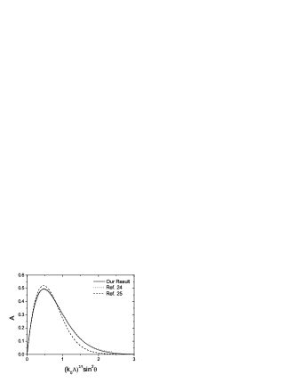
Figure 1: Mode conversion coefficient $\mathcal{A}$ as a function of $Q_{a}=\left(k_{0}\Lambda\right)^{2/3}\sin^{2}\theta$, for Model A. Our exact result is compared with the numerical result of Ref. 24 and the analytical result of Ref. 25.

In Fig. 1, we show the mode conversion coefficient as a function of the variable $Q_{a}$. In obtaining this result, we have used a sufficiently large $\tilde{L}$ ($\sim 100$) and a sufficiently small $\eta$ ($\sim 10^{-8}$) and the convergence was perfect. We compare our result with the numerical result of Ref. 24 and the analytical result of Ref. 25. We find that the agreement with Ref. 24 is very good, though we believe that the numerical accuracy of our result is better.

V Results on Model B: Linear density profile in half-space

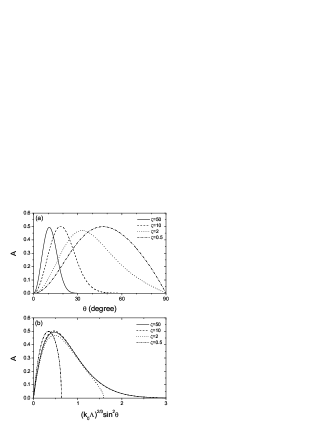
Figure 2: (a) Mode conversion coefficient $\mathcal{A}$ for Model B as a function of the incident angle $\theta$ for several values of $\zeta=k_{0}\Lambda$. (b) $\mathcal{A}$ as a function of $Q_{a}=\left(k_{0}\Lambda\right)^{2/3}\sin^{2}\theta$ for Model B. As $\zeta$ increases, the curves converge to the universal shape in Fig. 1.

In order to obtain the mode conversion coefficient in Model B, we solve the invariant imbedding equation for $r$ in Eq. (12) with the initial condition

$$r(0) = \frac{\left({\tilde{L}}-1\right)\cos\theta+i\sqrt{{\tilde{L}}-\cos^{2}\theta}}{\left({\tilde{L}}-1\right)\cos\theta-i\sqrt{{\tilde{L}}-\cos^{2}\theta}},$$ (19)

where we have used the values $\epsilon_{1}=1$ and $\epsilon_{2}=1-{\tilde{L}}$. In this case, the mode conversion coefficient is not a universal function of $Q_{a}$ even in the limit of ${\tilde{L}\rightarrow\infty}$ and $\eta\rightarrow 0$, since the linear density profile persists only in half-space. In Fig. 2, we show our exact results for several values of $\zeta=k_{0}\Lambda$ as functions of the incident angle $\theta$ and the parameter $Q_{a}$. As $\zeta$ increases, the curves converge to the universal shape in Fig. 1.

Figure 3: Absolute value of the magnetic field, $|B|$, as a function of $\left(z-z_{R}\right)/\Lambda$ for Model B, where $z_{R}$ ($\equiv L-\Lambda$) is the coordinate of the mode conversion point. $\zeta$ is equal to 12.5. (a) $\theta=5^{\circ}$ (b) $\theta=\sin^{-1}0.4\approx 23^{\circ}$ (c) $\theta=45^{\circ}$

We have also calculated the spatial dependence of the magnetic field amplitude $B(z)$ using the invariant imbedding equation (15). In Fig. 3, we plot the absolute value of the magnetic field amplitude, $|B|$, for $\zeta=12.5$ and several values of the incident angle $\theta$ as a function of $\left(z-z_{R}\right)/\Lambda$ where $z_{R}$ ($\equiv L-\Lambda$) is the coordinate of the mode conversion point. After a suitable rescaling of the variables, our Fig. 3(b) agrees quite well with Fig. 2(f) in Ref. 24.

VI Results on Model C: Parabolic density profile in entire space

The mode conversion in a warm, unmagnetized plasma with a parabolic density profile in entire space has been studied analytically by Hinkel-Lipsker et al..hink0 ; hink2 ; hink3 If we restrict our attention to the cold plasma case with zero temperature, our Model C is identical to the models studied in Refs. 26$-$28. In order to obtain the mode conversion coefficient, we solve the invariant imbedding equations for $r$ and $t$, Eq. (12), with the initial conditions $r(0)=0$ and $t(0)=1$. In the limit where ${\tilde{L}}\rightarrow\infty$ and $\eta\rightarrow 0$, we find numerically that the mode conversion coefficient ${\mathcal{A}}$ ($=1-|r|^{2}-|t|^{2}$) is a universal function of the parameters $Q_{c}\equiv k_{0}\Lambda\sin^{2}\theta/(1+\delta)^{1/2}$ and $\Delta^{2}\equiv k_{0}\Lambda\delta/(1+\delta)^{1/2}$. That this has to be the case can be seen by rewriting the wave equation using the variables introduced in Ref. 28, ${\overline{z}}\equiv{k_{0}}^{1/2}(1+\delta)^{1/4}z/\Lambda^{1/2}$, ${\overline{L}}\equiv{k_{0}}^{1/2}(1+\delta)^{1/4}L/\Lambda^{1/2}$, $\eta_{c}\equiv k_{0}\Lambda\eta/(1+\delta)^{1/2}$:

$${{{d^{2}}B}\over{d{\overline{z}}^{2}}}-\frac{2\left({\overline{z}}-{\overline{L}}/2\right)}{\left({\overline{z}}-{\overline{L}}/2\right)^{2}-\Delta^{2}+i\eta_{c}}{{dB}\over{d{\overline{z}}}}$$

$$~{}~{}~{}~{}+\left[\left({\overline{z}}-{\overline{L}}/2\right)^{2}-\Delta^{2}+i\eta_{c}-Q_{c}\right]B=0.$$ (20)

Figure 4: Absorption coefficient $\mathcal{A}$ for Model C as a function of $Q_{c}=k_{0}\Lambda\sin^{2}\theta$, for several values of the damping parameter $\eta_{c}$. The wave frequency is fixed at the peak plasma frequency, therefore $\delta$ is equal to zero. The value of $\tilde{L}$ used in the calculation is 400. Our exact result is compared with the analytical result of Ref. 27 represented by dashed lines.

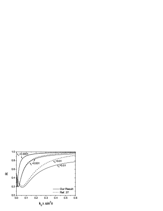
Figure 5: Reflectivity $\mathcal{R}$ for Model C as a function of $Q_{c}$, for several values of $\eta_{c}$. $\delta$ is zero and $\tilde{L}$ is 400. Our result is compared with that of Ref. 27 represented by dashed lines.

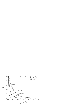
Figure 6: Transmissivity $\mathcal{T}$ for Model C as a function of $Q_{c}$, for several values of $\eta_{c}$. $\delta$ is zero and $\tilde{L}$ is 400. Our result is compared with that of Ref. 27 represented by dashed lines.

When the wave frequency is equal to the local plasma frequency at the top of the parabolic density profile, corresponding to $\delta=0$, the quantity $\mathcal{A}$ vanishes unless $\eta_{c}>0$ and there is no true mode conversion. In this case, we will call $\mathcal{A}$, which measures the absorption due to collisional damping, as the absorption coefficient instead of the mode conversion coefficient.

In Figs. 4, 5 and 6, we show the absorption coefficient, the reflectivity and the transmissivity when $\delta=0$ as a function of the parameter $Q_{c}$ for several values of $\eta_{c}$. The scaled thickness of the plasma $\tilde{L}$ used in the calculation is equal to 400. Our numerically exact results are compared with those in Ref. 27. The agreement is quite good when $\eta_{c}=0.0001$, but becomes worse as $\eta_{c}$ increases. In fact, if we do the calculation for larger $\tilde{L}$ values, we find our absorption coefficient gets bigger and the discrepancy between our result and that of Ref. 27 increases gradually. This is reasonable because the damping occurs in the entire region of thickness $\tilde{L}$ in our calculation, whereas several approximations limiting the effects of damping to a small region surrounding the peak point have been made in Ref. 27. We have calculated the absorption coefficient for the cases where the damping parameter $\eta_{c}$ is nonzero only in a narrow region of small width surrounding the point $z=L/2$. The discrepancy between the result of this calculation and that of Ref. 27 is much smaller than in Fig. 4, but there is no unique way of choosing a particular width.

Figure 7: Absorption coefficient when the angle of incidence is zero, $\mathcal{A}(\theta=0)$, for Model C as a function of the damping parameter $\eta_{c}$. $\delta$ is zero and $\tilde{L}$ is 400.

In Fig. 7, we plot the value of the absorption coefficient when the angle of incidence is zero as a function of the damping parameter. $\delta$ is zero and $\tilde{L}$ is 400. We find an almost linear increase of $\mathcal{A}(\theta=0)$, whereas it remains zero in Ref. 27.

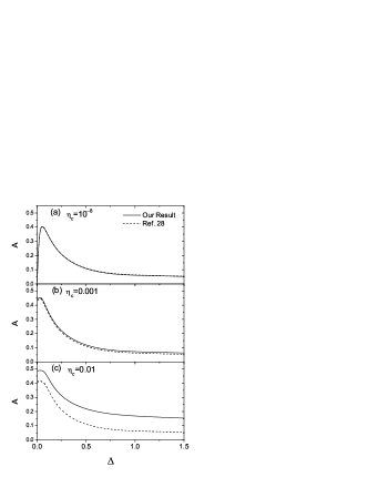
Figure 8: Absorption coefficient $\mathcal{A}$ for Model C as a function of the parameter $\Delta$ for several values of $\eta_{c}$. $Q_{c}$ is 0.05 and $\tilde{L}$ is 400. Our result is compared with that of Ref. 28 represented by dashed lines. (a) $\eta_{c}=10^{-8}$ (b) $\eta_{c}=0.001$ (c) $\eta_{c}=0.01$

In Fig. 8, we show the absorption coefficient as a function of the parameter $\Delta$ for several values of the damping parameter. $\tilde{L}$ is 400 and $Q_{c}$ is 0.05. Our exact result is compared with the analytical result of Ref. 28. The agreement is quite good when $\eta_{c}=10^{-8}$, but becomes worse as $\eta_{c}$ increases for the same reason as in Figs. 4, 5 and 6. If $\Delta$ is nonzero, the wave frequency is shifted from the peak plasma frequency and the mode conversion occurs at two points, $z=L/2\pm\left[\delta/\left(\delta+1\right)\right]^{1/2}\Lambda$, where $\delta$ is related to $Q_{c}$ and $\Delta$ by $\delta=\left(\Delta^{2}\sin^{2}\theta\right)/Q_{c}$. For a finite $\eta_{c}$, the quantity $\mathcal{A}$ includes the absorption due to both collisional damping and mode conversion. As $\eta_{c}$ approaches zero, $\mathcal{A}$ becomes the genuine mode conversion coefficient. The curve in Fig. 8(a) is a well-converged one which shows only the absorption due to mode conversion. The differences between Fig. 8(a) and Figs. 8(b) and 8(c) represent the absorption due to collisional damping.

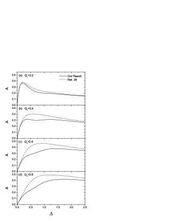
Figure 9: Mode conversion coefficient $\mathcal{A}$ for Model C as a function of the parameter $\Delta$ for several values of $Q_{c}$. $\eta_{c}$ is $10^{-8}$ and $\tilde{L}$ is 400. Our result is compared with that of Ref. 28 represented by dashed lines. (a) $Q_{c}=0.2$ (b) $Q_{c}=0.4$ (c) $Q_{c}=0.6$ (d) $Q_{c}=0.8$

In Fig. 9, we plot the mode conversion coefficient, which is the absorption coefficient in the $\eta_{c}\rightarrow 0$ limit, as a function of $\Delta$ for several values of $Q_{c}$. The values of $\tilde{L}$ and $\eta_{c}$ used in the calculation are 400 and $10^{-8}$ respectively. We have verified that these results are well-converged in the sense that the results of the calculation for $\tilde{L}$ values bigger than 400 and $\eta_{c}$ values smaller than $10^{-8}$ are indistinguishable from those shown in Fig. 9. We believe this is the first exact calculation of the mode conversion coefficient in the parabolic case. Our exact result is compared with the analytical formulas of Ref. 28. Unlike the $Q_{c}=0.05$ case shown in Fig. 8(a), the discrepancy between our result and that of Ref. 28 is sizable. The shape of the curves is not very simple. For instance, we observe a double-peaked structure in Fig. 9(b).

VII Conclusion

In this paper, we have presented a new version of the invariant imbedding theory of the wave propagation in stratified media and applied it to the mode conversion phenomena of $p$ waves in cold, unmagnetized plasmas. We have obtained the mode conversion coefficient and the field distribution exactly for linear and parabolic plasma density profiles for the first time. Using a recent generalization of the invariant imbedding theory for the propagation of coupled waves in stratified media, we can apply our method to more general situations in a straightforward manner.kim3 In forthcoming papers, we will present the result of our study on the mode conversion in magnetized plasmas and the temperature effects on both unmagnetized and magnetized plasmas.

- (1) K. G. Budden, The Propagation of Radio Waves (Cambridge University Press, Cambridge, 1985).
- (2) V. L. Ginzburg, The Propagation of Electromagnetic Waves in Plasmas (Pergamon, New York, 1970).
- (3) D. G. Swanson, Theory of Mode Conversion and Tunneling in Inhomogeneous Plasmas (Wiley, New York, 1998).
- (4) T. H. Stix, Waves in Plasmas (AIP Press, New York, 1992).
- (5) E. Mjølhus, Radio Sci. 25, 1321 (1990).
- (6) T. H. Stix, Phys. Rev. Lett. 15, 878 (1965).
- (7) B. N. Moore and M. E. Oakes, Phys. Fluids 15, 144 (1972).
- (8) L. Chen and A. Hasegawa, J. Geophys. Res. 79, 1024 (1974).
- (9) W. Woo, K. Estabrook, and J. S. DeGroot, Phys. Rev. Lett. 40, 1094 (1978).
- (10) R. A. Cairns and C. N. Lashmore-Davies, Phys. Fluids 26, 1268 (1983).
- (11) A. K. Ram, A. Bers, S. D. Schultz, and V. Fuchs, Phys. Plasmas 3, 1976 (1996).
- (12) P. M. Bellan, J. Geophys. Res. 101, 24887 (1996).
- (13) L. Yin and M. Ashour-Abdalla, Phys. Plasmas 6, 449 (1999).
- (14) J. R. Johnson, T. Chang, and G. B. Crew, Phys. Plasmas 2, 1274 (1995).
- (15) J. R. Johnson, C. Z. Cheng, and P. Song, Geophys. Res. Lett. 28, 227 (2001).
- (16) A. J. Wiles and I. H. Cairns, Phys. Plasmas 10, 4072 (2003).
- (17) D.-H. Lee, M. K. Hudson, K. Kim, R. L. Lysak, and Y. Song, J. Geophys. Res. 107, 1307 (2002).
- (18) D.-H. Lee and K. Kim, J. Korean Phys. Soc. 40, 353 (2002).
- (19) N. G. Denisov, Sov. Phys. JETP 4, 544 (1951).
- (20) A. D. Piliya, Sov. Phys. Tech. Phys. 11, 609 (1966).
- (21) T. Speziale and P. J. Catto, Phys. Fluids 20, 990 (1977).
- (22) G. J. Pert, Plasma Phys. 20, 175 (1978).
- (23) R. W. Means, L. Muschietti, M. Q. Tran, and J. Vaclavik, Phys. Fluids 24, 2197 (1981).
- (24) D. W. Forslund, J. M. Kindel, K. Lee, E. L. Lindman, and R. L. Morse, Phys. Rev. A 11, 679 (1975).
- (25) D. E. Hinkel-Lipsker, B. D. Fried, and G. J. Morales, Phys. Fluids B 4, 559 (1992).
- (26) D. E. Hinkel-Lipsker, B. D. Fried, and G. J. Morales, Phys. Rev. Lett. 66, 1862 (1991).
- (27) D. E. Hinkel-Lipsker, B. D. Fried, and G. J. Morales, Phys. Fluids B 4, 1772 (1992).
- (28) D. E. Hinkel-Lipsker, B. D. Fried, and G. J. Morales, Phys. Fluids B 5, 1746 (1993).
- (29) R. Bellman and G. M. Wing, An Introduction to Invariant Imbedding (Wiley, New York, 1976).
- (30) V. I. Klyatskin, Prog. Opt. 33, 1 (1994).
- (31) N. V. Gryanik and V. I. Klyatskin, Sov. Phys. JETP 84, 1106 (1997).
- (32) R. Rammal and B. Doucot, J. Phys. (Paris) 48, 509 (1987).
- (33) K. Kim, Phys. Rev. B 58, 6153 (1988).
- (34) K. Kim, H. Lim, and D.-H. Lee, J. Korean Phys. Soc. 39, L956 (2001).
- (35) K. Kim, D.-H. Lee, and H. Lim, Europhys. Lett. 69, 207 (2005).