Numerical Solution of the 1D Schrödinger Equation: Bloch Wavefunctions

Abstract

In this article we discuss a procedure to solve the one dimensional (1D) Schrödinger Equation for a periodic potential, which may be well suited to teach band structure theory. The procedure is conceptually very simple, so that it may be used to teach band theory at the undergraduate level; at the same time the point of view is practical, so that the students may experiment computing band gaps, and other features of band structure. Another advantage of the procedure lies in that it does not use specific symmetry properties of the potential, so that the results are generally valid.

I Introduction

Most traditional textbooks dealing with Solid State Theory at an elementary level discuss the fundamentals of band structure calculations, including in most cases only a theoretical description of the essential features of band structure, usually with a discussion of the Kronnig-Penney model Neil Ashcroft and N. David Mermin (1976). Of course, this is of great pedagogical value, but presenting only this viewpoint is unsatisfactory, given the great amount of computer resources available today, and the relative ease with which one may take advantage of the added insight that may be obtained from simple numerical calculations.

Of course, this fact has not been neglected in scientific literature; many articles have been devoted to the numerical solution of the Schrödinger equation in this and other journals A.A. Bahurmuz and P.D. Loly (1981); Sami A. Shakir (1983); R. T. Deck and Xiangshan Li (1995); S.A. Denham, B.C. Harms and S. T. Jones (1982); Juan F. Van der Maelen Uría, Santiago García-Granda and Amador Menéndez-Velásquez (1996); Leung (1993); B. Méndez and F. Domínguez-Adame (1994); R. C. Greenhow and J. A. D. Mathew (1992); Johnston (1992); P. J. Cooney, E. P. Kanter and Z. Vager (1981); Debra J. Searles and Ellak I. von Nagy-Felsobuki (1988). The references cited here intend only to be a (biased) sample of the large existing literature on the subject of numerically solving the Schrödinger equation for one dimensional potentials. Most of the articles seem to concentrate on the problem of finding bound states Sami A. Shakir (1983); S.A. Denham, B.C. Harms and S. T. Jones (1982); Juan F. Van der Maelen Uría, Santiago García-Granda and Amador Menéndez-Velásquez (1996); R. C. Greenhow and J. A. D. Mathew (1992); P. J. Cooney, E. P. Kanter and Z. Vager (1981); Debra J. Searles and Ellak I. von Nagy-Felsobuki (1988), while a relatively minor number treat the problem of finding the energy spectra for a periodic potential A.A. Bahurmuz and P.D. Loly (1981); R. T. Deck and Xiangshan Li (1995); Leung (1993); B. Méndez and F. Domínguez-Adame (1994); Johnston (1992), which is the subject of this article.

The band theory of Bloch electrons in a periodic potential is basic for an understanding of solid state physics. The usual description is given in most texts in solid state theory(see, for example Aschcroft and Mermin’s classic textbook Neil Ashcroft and N. David Mermin (1976), which we follow here for the one dimensional case.

Consider an electron (mass $m$) moving in a periodic potential $U(x+a)=U(x)$, in which the potential $U(x)$ is written as a superposition of potential barriers $v(x)$, centered the points $x=\pm(n+1/2)a$:

$$U(x)=\sum_{n=-\infty}^{\infty}v(x-na).$$ (1)

The band structure of the one dimensional solid is expressed in terms of the properties of an electron scattering from a single potential barrier $v(x)$. Therefore, they (Neil Ashcroft and N. David Mermin (1976)) write the wavefunction for an electron scattering from the left, with energy $E=\hbar^{2}K^{2}/2m$, in terms of reflection and transmission amplitudes $r$ and $t$; these wavefunction become, for $x>a$

$$\Psi_{l}(x) = e^{iKx}+re^{-iKx},~{}~{}x<0$$ (2)

$$= te^{iKx},~{}~{}x>a,$$

while, for the electron coming from the right-hand side, the wavefunction is

$$\Psi_{r}(x) = te^{-iKx},~{}~{}x<0$$ (3)

$$= e^{-iKx}+re^{iKx},~{}~{}x>a.$$

Observe that these results are valid only for a potential that is even with respect to $x=a/2$, otherwise, one would have to introduce different coefficients $r^{\prime}$ and $t^{\prime}$ in the last equation. We assume, of course, that the rest of the solutions, i.e., the part corresponding to the region $0<x<a$ has been found by some procedure. Clearly, since $\Psi_{l}$ and $\Psi_{r}$ are two independent solutions of the Schrödinger equation corresponding to the same energy, the full solution of the Schrödinger equation corresponding to the periodic solid will be expressed as a the linear combination (now for $0<x<a$)

$$\Psi(x)=A\Psi_{l}(x)+B\Psi_{r}(x),~{}~{}0<x<a.$$ (4)

According to Bloch’s Theorem, the wavefunction $\Psi(x)$ satisfies the relation

$$\Psi(x+a)=e^{ika}\Psi(x),$$ (5)

for suitable values of $k$. The same relations holds for the derivative of $\Psi(x)$, namely

$$\Psi^{\prime}(x+a)=e^{ika}\Psi^{\prime}(x).$$ (6)

Imposing the conditions above on the wavefunction $\Psi(x)$, gives a relation that may be used to obtain the energy vs. wavevector relation $E=E(k)=\hbar^{2}K^{2}/2m$,

$$\cos(ka)=\frac{t^{2}-r^{2}}{2t}e^{iKa}+\frac{1}{2t}e^{-iKa}.$$ (7)

It is then shown that the energy is a periodic function of the Bloch wavenumber $k$, with period $G=2\pi/a$ (the reciprocal lattice vector).

$$E_{k+G}=E_{k}$$ (8)

Let us concentrate on the solution of the equation for the Bloch wavefunction $u(x)$. One way to do this may be to expand the wavefunction $\Psi$ in a Fourier series, doing the same for the potential, namely

$$\Psi(x) = \sum_{q}c_{q}e^{iqx}$$

$$U(x) = \sum_{G}U_{G}~{}e^{iGx}$$

$$U_{G} = \frac{1}{a}\int_{0}^{a}e^{-iGx}U(x)dx,$$

in which the $U_{G}$ are Fourier coefficients, and the sum over $G$ goes over reciprocal lattice vectors.

The equation for the coefficients $c_{q}$ is customarily written as follows

$$\left(\frac{\hbar^{2}}{2m}(k-G)^{2}-E\right)c_{k-G}+\sum_{G^{\prime}}U_{G^{\prime}-G}c_{k-G^{\prime}}=0.$$ (9)

From a numerical point of view, this equation may be slow in converging to an accurate solution, one may need to include a large number of terms in the resulting matrix equation. However, this method has been successfully used to calculate band structures of real solids (3D).

In the 1D case, we have other methods at our disposal, which may be better suited to the problem. Unfortunately, most of the methods available for the 1D case cannot be taken over to the 3D case, and our proposal is not an exception to this (alas!).

II Numerical Solution

Now let us discuss the particular situation that arises in 1D. A peculiarity of our treatment is that we really have no need for the auxiliary function $u(x)$, as it will be seen presently.

Now, to actually find numerical solutions of the Schrödinger equation, and the corresponding energies, we proceed as follows. For each value of the energy $E$, considered here as a parameter, we find two independent numerical solutions, which we call $C(x)$ and $S(x)$. For example, for a fundamental period with endpoints at $x=0$ and $x=a$, these functions may be chosen to satisfy

$$C(a/2)=1 C^{\prime}(a/2)=0$$ (10)

$$S(a/2)=0 S^{\prime}(a/2)=1$$ (11)

To numerically obtain the functions $C$ and $S$ we divide the integration region in two regions, $0<x<a/2$, and $a/2<x<a$. We start the integration from the center ( $x=a/2$ towards the boundaries of the two regions, imposing at the start the continuity of the function ( $C$ os $S$). After this is done, we compute the normalization integral, $N=\int_{0}^{a}|\Psi(x)|^{2}dx$ and redefine the function, dividing by $\sqrt{N}$. Observe that the wavefunction defined in this way, be it $C$ or $S$, does not satisfy the full boundary conditions: it is a real function, and it may not even be periodic, the boundary conditions are satisfied only by the full wavefunction $\Psi(x)$. For the numerical integration, I have used the Numerov P. C. Chow (1972) procedure, since it is very accurate and simple to use, however, any reliable numerical method may be used just as easily, such as Runge-Kutta, with or without adaptive step size W. H. Press, B. P. Flannery, S. A. Teukolsky and W. P. Vetterling (1989).

The functions $C(x)$ and $S(x)$ are actually dependent upon the energy $E$, i.e., $C(x)=C_{E}(x)$ and $S(x)=S_{E}(x)$, but to make the notation less cumbersome, we drop the parameter $E$ henceforth, unless it is necessary to keep it. The full wavefunction must be expressed as a the linear combination of the functions $C$ and $S$, with possibly complex coefficients $A$ and $B$, the only way to satisfy the boundary conditions from our purely real basis functions $C$ and $S$,

$$\Psi(x)=A\cdot C(x)+B\cdot S(x).$$ (12)

The boundary conditions are now

$$\Psi(a)=e^{ika}\Psi(0)$$

$$\Psi^{\prime}(a)=e^{ika}\Psi^{\prime}(0),$$ (13)

which may be written as equations for the coefficients $A$ and $B$,

$$\Delta_{C}A+\Delta_{S}B = 0$$

$$\Delta_{C}^{\prime}A+\Delta_{S}^{\prime}B = 0,$$ (14)

in which the coefficients are may be written as (using $\theta=ka/2$)

$$\Delta_{C} = e^{i\theta}C(a)-e^{-i\theta}C(0)$$

$$\Delta_{S} = e^{i\theta}S(a)-e^{-i\theta}S(0)$$

$$\Delta_{C}^{\prime} = e^{i\theta}C^{\prime}(a)-e^{-i\theta}C^{\prime}(0)$$

$$\Delta_{S}^{\prime} = e^{i\theta}S^{\prime}(a)-e^{-i\theta}S^{\prime}(0)$$ (15)

The equation for the energies is then given by the vanishing of the determinant of the coefficients,

$$G(E)=\Delta_{C}\Delta_{S}^{\prime}-\Delta_{S}\Delta_{C}^{\prime}=0$$ (16)

When, as in our case, the potential is symmetric with respect to the midpoint of the period, the functions $C$ and $S$ have definite parity about that point, i.e. $C(a)=C(0)$ and $S(a)=-S(0)$. Also, the derivatives have the opposing parity, $C^{\prime}(a)=-C^{\prime}(0)$ and $S^{\prime}(a)=S^{\prime}(0)$, therefore,

$$\Delta_{C} = 2i\sin(\theta)C(0)$$

$$\Delta_{S} = -2\cos(\theta)S(0)$$

$$\Delta_{C}^{\prime} = -2\cos(\theta)C^{\prime}(0)$$

$$\Delta_{S}^{\prime} = 2i\sin(\theta)S^{\prime}(0)$$ (17)

The eigenvalue equation becomes

$$G(E)=\sin^{2}(\theta)C(0)S^{\prime}(0)+\cos^{2}(\theta)S(0)C^{\prime}(0)=0$$ (18)

These equations are convenient for numerical work, since the functions $C$ and $S$ are easily computed numerically, and the left hand side of the equation may be plotted, as a function of $E$, the zeros being the eigenstates that we are looking for.

In the general (non symmetric) case, we can write

$$\Delta_{C} = [C(a)-C(0)]\cos(\theta)+i[C(a)+C(0)]\sin(\theta)$$

$$\Delta_{S} = [S(a)-S(0)]\cos(\theta)+i[S(a)+S(0)]\sin(\theta)$$

$$\Delta_{C}^{\prime} = [C^{\prime}(a)-C^{\prime}(0)]\cos(\theta)+i[C^{\prime}(a)+C^{\prime}(0)]\sin(\theta)$$

$$\Delta_{S}^{\prime} = [S^{\prime}(a)-S^{\prime}(0)]\cos(\theta)+i[S^{\prime}(a)+S^{\prime}(0)]\cos(\theta)$$ (19)

Now, let

$$C_{(-)} = C(a)-C(0)$$

$$C_{(+)} = C(a)+C(0)$$

$$S_{(-)} = S(a)-S(0)$$

$$S_{(+)} = S(a)+S(0)$$

$$C^{\prime}_{(-)} = C^{\prime}(a)-C^{\prime}(0)$$

$$C^{\prime}_{(+)} = C^{\prime}(a)+C^{\prime}(0)$$

$$S^{\prime}_{(-)} = S^{\prime}(a)-S^{\prime}(0)$$

$$S^{\prime}_{(+)} = S^{\prime}(a)+S^{\prime}(0).$$

We obtain, for the real and imaginary parts of the eigenvalue equation:

$$\Re[G(E)] = \left(C_{(-)}S^{\prime}_{(-)}-S_{(-)}C^{\prime}_{(-)}\right)\cos^{2}(\theta)$$

$$+ \left(S_{(+)}C^{\prime}_{(-)}-C_{(+)}S^{\prime}_{(-)}\right)\sin^{2}(\theta)$$

$$\Im[G(E)] = \left(C_{(-)}S^{\prime}_{(+)}+C_{(+)}S^{\prime}_{(-)}-S_{(-)}C^{\prime}_{(+)}-S_{(+)}C^{\prime}_{(-)}\right)$$

$$\times \sin(\theta)\cos(\theta)$$

First, concentrate upon computing the terms of the $\Im(G)$, they become

$$C_{(-)}S^{\prime}_{(+)}+C_{(+)}S^{\prime}_{(-)} = 2[C(a)S^{\prime}(a)-C(0)S^{\prime}(0)]$$

$$S_{(-)}C^{\prime}_{(+)}+S_{(+)}C^{\prime}_{(-)} = 2[S(a)C^{\prime}(a)-S(0)C^{\prime}(0)]$$

Putting all this together, we find

$$\Im(G(E))=2\sin(\theta)\cos(\theta)\left(W[C,S](a)-W[C,S](0)\right),$$ (20)

where $W[C,S](\phi=C(\phi)S^{\prime}(\phi)-C^{\prime}(\phi)S(\phi)$ is the Wronskian of the solutions $C$ and $S$; moreover, a well known theorem tells us that the Wronskian is a constant, as it may easily shown, hence, we have shown that the imaginary part of $G$ identically vanishes

$$\Im[G(E)]=0.$$ (21)

The eigenvalue equation is therefore,

$$G(E) = \left(C_{(-)}S^{\prime}_{(-)}-S_{(-)}C^{\prime}_{(-)}\right)\cos^{2}(\theta)$$

$$+ \left(S_{(+)}C^{\prime}_{(-)}-C_{(+)}S^{\prime}_{(-)}\right)\sin^{2}(\theta)$$

III Simple Examples

As indicated previously, a numerical calculation such as the one proposed here is able to give us all the energy bands that we care to compute (with due consideration of the limitations of each integration method). Since computing wavefunctions is relatively ’cheap’, we have developed a computer program that does the following:

1. Divides the first Brillouin zone in $N$ intervals of size $\Delta k=2\pi/Na$.

2. Prompts the user to indicate the energy range, from $E_{min}=min(V(x)$, $0<x<a$) to $E_{max}$. The energy interval is divided into $N_{E}$ subintervals, of size $\Delta E=(E_{max}-E_{min})/N_{E}$.

3. For each fixed value of the wavenumber $k=k_{0}$, it computes the normalized basis functions $C$ and $S$. From these, it computes the function $G(E_{i})$, at each of the $N_{E}$ points of the energy interval. These values are sent to an array (and stored in a file).

4. The program seeks the roots of the equation $G(E)=0$, using the values obtained previously as a starting point; the energies are then refined by a combination of Newton’s method (actually, the Secant method) and bisection.

5. The resulting roots are stored in a file. Next, move over to the next value of $k$ in the $k$-grid ($k=k_{0}+\Delta k$), and repeat the previous step. Since this is done for each value of $k=k_{j}=k_{0}+j\Delta k$, one obtains the band structure directly from this calculation.

As numerical examples, we show the results obtained for three simple potentials, with period $2\pi$:

• The Kronig-Penney model (with $V_{0}=1$, width $a=0.5$ centered at $x=\pi$)

  $$V(x) = 0,~{}~{}for~{}~{}|x-\pi|>a$$ (22)

  $$= V_{0}~{}~{}for~{}~{}|x-\pi|<a,$$

• the sinusoidal potential (with $V_{0}=1$ also),

  $$V(x)=V_{0}(1-cos(x))/2,$$ (23)

• and a triangular potential,

  $$V(x) = V_{0}(\pi-x)/\pi,~{}~{}for~{}~{}x<\pi$$ (24)

  $$= V_{0}(x-\pi)/\pi~{}~{}for~{}~{}x>\pi.$$

These potentials are plotted together in Figure 1, we have chosen them to have the same maxima, minima, and fundamental period $0<x<2\pi$. These potentials have all been thoroughly studied in the literature: the Kronig-Penney model has solutions that may be expressed in terms of sinusoidal and exponential functions. The energy vs. wavenumber relation, $E(k)$, however, is a trascendental equation; its solution must be obtained numerically, which somewhat offsets the comparative ease with which one obtains the wavefunctions. As described in Stiddard’s textbook M. H. B. Stiddard (1975) ( in his notation: a square barrier, of width $a$, period $a+b$), the eigenvalue equation is

$$\frac{\gamma^{2}-\beta^{2}}{2\beta\gamma}sinh(\gamma b)\sin(\beta a)+cosh(\gamma b)\cos(\beta a)=cos(k(a+b)).$$ (25)

The triangular potential may also be solved analitically, in terms of Airy functions, but the eigenvalue equation becomes very cumbersome to evaluate. A similar situation occurs for the sinusoidal potential, which solutions may be expressed in terms of Mathieu functions. In all cases, the analytical calculations needed to obtain the eigenvalue equation from the boundary conditions become very involved; much more involved that the numerical solutions described here, and the ’icing on the cake’, so to speak, is the fact that in the end, all has to be evaluated numerically. So, why not do it numerically from begining to end?. The results of our calculations are shown in Figure 2.

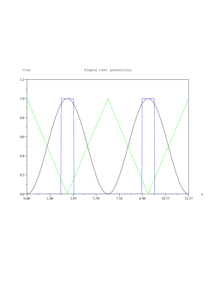
Figure 1: The test potentials used in this work: sinusoidal potential $(1-cos(x))/2$, Kronig-Penney potential centered at $x=\pi$, and a triangular potential.

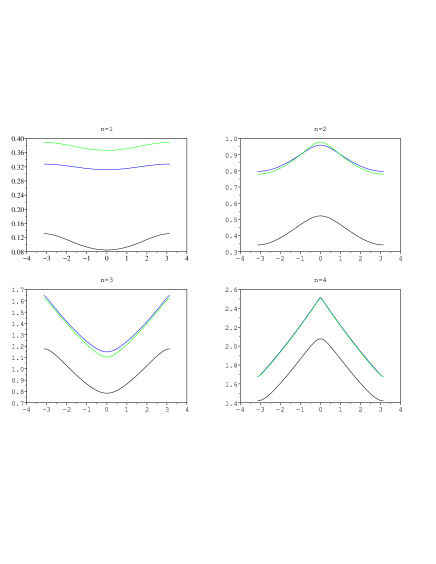
Figure 2: First four energy bands for the three model potentials. The Kronig-Penney potential is shown in the black curve, the sinusoidal potential in the blue curve, and the triangular potential on the green curve.

IV Final comments

First, we have established a simple numerical procedure that enables us to compute numerically the wavefunctions and energy vs. wavevector curve, $E(k)$ for any periodic potential. The procedure is very simple, yet it appears that it has not been discussed previously, enabling us to study the effect that a parameter change on the potential has on the energies $E(k)$, band gaps and densities of states $g(E)$. The procedure may be implemented quite simple using Matlab or Scilab.