Multifractality of Inverse Statistics of Exit Distances in 3D Fully Developed Turbulence

Abstract

The inverse structure functions of exit distances have been introduced as a novel diagnostic of turbulence which emphasizes the more laminar regions Jensen (1999); Roux and Jensen (2004); Biferale et al. (2001, 2003). Using Taylor’s frozen field hypothesis, we investigate the statistical properties of the exit distances of empirical 3D fully developed turbulence. We find that the probability density functions of exit distances at different velocity thresholds can be approximated by stretched exponentials with exponents varying with the velocity thresholds below a critical threshold. We show that the inverse structure functions exhibit clear extended self-similarity (ESS). The ESS exponents $\xi(p,2)$ for small $p$ ($p<3.5$) are well captured by the prediction of $\xi(p,2)=p/2$ obtained by assuming a universal distribution of the exit distances, while the observed deviations for large $p$’s characterize the dependence of these distributions on the velocity thresholds. By applying a box-counting multifractal analysis of the natural measure constructed on the time series of exit distances, we demonstrate the existence of a genuine multifractality, endowed in addition with negative dimensions. Performing the same analysis of reshuffled time series with otherwise identical statistical properties for which multifractality is absent, we show that multifractality can be traced back to non-trivial dependence in the time series of exit times, suggesting a non-trivial organization of weakly-turbulent regions.

I Introduction

In isotropic turbulence, structure functions are among the favorite statistical indicators of intermittency. The (longitudinal) structure function of order $p$ is defined by $S_{p}({r})\equiv\langle\delta{v}_{\parallel}({r})^{p}\rangle$. The K41 theory Kolmogorov (1941) obtains that $S_{p}({r})=C_{p}\epsilon^{p/3}{r}^{p/3}$, where $\epsilon$ is the average energy dissipation rate of the fluid element of size ${r}$ and $C_{p}$ is a constant independent of Reynolds number. The K62 theory Kolmogorov (1962) extends K41 by assuming a log-normal distribution of $\epsilon$, which was questioned by Mandelbrot Mandelbrot (1972). The anomalous scaling properties was uncovered experimentally Anselmet et al. (1984) implying the non-Gaussianity of the probability distribution of the velocity increments.

The velocity structure functions consider the moments of velocity increments over space. However, when one turns to the scalar statistics in passive scalar advection, one often considers averages of the advection time versus the distance Frisch et al. (1998); Gat et al. (1998). An alternative quantity was introduced, denoted the distance structure functions Jensen (1999) or inverse structure functions Biferale et al. (1999, 2001):

$$T_{p}(\delta v)\equiv\langle{{r}^{p}(\delta v)}\rangle,$$ (1)

where $\delta v$ are a set of pre-chosen thresholds of velocity increments and ${r}(\delta v)$ is the exit distance defined as the minimal distance for the velocity difference to exceed $\delta{v}$

$${r}(\delta v)=\inf\left\{r:|v_{i\pm r}-v_{i}|>\delta{v}\right\}~{},$$ (2)

given a record of velocity $v_{i}$. In the literature, alternative definitions are adopted as well, such as $|v_{i+r}-v_{i}|>\delta{v}$ or $v_{i+r}-v_{i}>\delta{v}$.

To ensure that the exit distance is defined, the threshold $\delta v$ should be less than $\delta v_{\max}=(v_{\max}-v_{\min})/2$, where $v_{\max}$ and $v_{\min}$ are respectively the maximum and minimum of the record. On the other hand, there is a minimal velocity increment $\delta v_{\min}=\min(|v_{i+1}-v_{i}|)$ for a given record such that for any $\delta v\leq\delta v_{\min}$ we have ${r}=1$. Therefore, we consider the range $(\delta{v}_{\min},\delta{v}_{\max})$. For any $\delta{v}$ in this range, by construction, we will obtain finite ${r}$ values from the velocity record.

The statistical properties studied for synthetic data of 24630 situations from the GOY shell model of turbulence exhibit perfect scaling dependence of the inverse structure functions on the velocity threshold Jensen (1999). A completely different result was obtained in Biferale et al. (1999) where an experimental signal was analyzed and no clear scaling was found in the exit distance structure functions. For smoother stochastic fluctuations associated with a spectrum with exponent $3\leq\beta<5$, such as two-dimensional turbulence, the inverse structure functions exhibit bifractality Biferale et al. (2001). While the large $\delta{v}$’s at fixed ${r}$ of the velocity structure functions emphasize the most intermittent region in turbulence, the large ${r}$’s at fixed $\delta{v}$ probe the laminar regions. Hence, the inverse structure functions provide probes of the intermediate dissipation range (IDR) Biferale et al. (1999) introduced in Frisch and Vergassola (1991). It is clear that the extreme events in the distribution of ${r}$ provide the prevailing contributions to the inverse structure functions for large exponents, which should thus be investigated carefully.

To our knowledge, inverse structure functions (or equivalently the statistics of exit distances) have not been used to characterize experimental three-dimensional turbulence data. Here, we describe in detail the probability distribution of exit distances ${r}$ and find that the stretched exponential distribution is a good approximation for all ${r}$’s. Then, we analyze the convergence of the inverse structure functions and investigate their multiscaling properties. We construct a measure based on the exit distance at each level $\delta{v}$ and unveil the multifractal nature of the measure.

II Standard preliminary tests on the experimental data

Very good quality high-Reynolds turbulence data have been collected at the S1 ONERA wind tunnel by the Grenoble group from LEGI Anselmet et al. (1984). We use the longitudinal velocity data obtained from this group. The size of the velocity time series we analyzed is $N\approx 1.73\times 10^{7}$.

The mean velocity of the flow is approximately $\langle{v}\rangle=20$m/s (compressive effects are thus negligible). The root-mean-square velocity fluctuations is $v_{\mathtt{rms}}=1.7$m/s, leading to a turbulence intensity equal to $I={v_{\mathtt{rms}}}/{\langle{v}\rangle}=0.0826$. This is sufficiently small to allow for the use of Taylor’s frozen flow hypothesis. The integral scale is approximately $4\mathtt{m}$ but is difficult to estimate precisely as the turbulent flow is neither isotropic nor homogeneous at these large scales.

The Kolmogorov microscale $\eta$ is given by Meneveau and Sreenivasan (1991) $\eta=\left[\frac{\nu^{2}\langle{v}\rangle^{2}}{15\langle(\partial v/\partial t)^{2}\rangle}\right]^{1/4}=0.195\mathtt{mm}$, where $\nu=1.5\times 10^{-5}\mathtt{m^{2}s^{-1}}$ is the kinematic viscosity of air. $\partial v/\partial t$ is evaluated by its discrete approximation with a time step increment $\partial t=3.5466\times 10^{-5}\mathtt{s}$ corresponding to the spatial resolution $\delta_{r}=0.72\mathtt{mm}$ divided by $\langle{v}\rangle$.

The Taylor scale is given by Meneveau and Sreenivasan (1991) $\lambda=\frac{\langle{v}\rangle v_{\mathtt{rms}}}{\langle(\partial v/\partial t)^{2}\rangle^{1/2}}=16.6\mathtt{mm}$. The Taylor scale is thus about $85$ times the Kolmogorov scale. The Taylor-scale Reynolds number is $Re_{\lambda}=\frac{v_{\mathtt{rms}}\lambda}{\nu}=2000$. This number is actually not constant along the whole data set and fluctuates by about $20\%$.

We have checked that the standard scaling laws previously reported in the literature are recovered with this time series. In particular, we have verified the validity of the power-law scaling $E(k)\sim k^{-\beta}$ with an exponent $\beta$ very close to $\frac{5}{3}$ over a range more than two decades, similar to Fig. 5.4 of Frisch (1996) provided by Gagne and Marchand on a similar data set from the same experimental group. Similarly, we have checked carefully the determination of the inertial range by combining the scaling ranges of several velocity structure functions (see Fig. 8.6 of (Frisch, 1996, Fig. 8.6)). Conservatively, we are led to a well-defined inertial range $60\leq{r}/\eta\leq 2000$.

III Scaling properties of inverse structure functions

III.1 The probability distributions of exit distances

We have obtained the exit times for 26 $\delta{v}$ values: 0.01, 0.0178, 0.0316, 0.0562, 0.1, 0.2, 0.3, 0.4, 0.5, 0.6, 0.7, 0.8, 0.9, 1, 1.1, 1.2, 1.3, 1.4, 1.5, 1.6, 1.7, 1.8, 1.9, 2, 2.33, and 2.7144 m/s. Fig. 1 shows the probability density functions (pdf’s) $P(r)$ as a function of $r/\sigma$ for different velocity thresholds $\delta v=0.5$m/s ($\Box$), $\delta v=1$m/s ($\ast$), $\delta v=1.5$m/s ($\triangleleft$) and $\delta v=2$m/s ($\star$), where $\sigma^{2}=\langle r^{2}\rangle$ is a function of $\delta{v}$. It is natural to normalize the exit distances by their standard deviation $\sigma(\delta v)$ for a given $\delta v$ and obtain the pdf of these normalized exit distances $x=r/\sigma$ as

$$\Phi(x)=\sigma P(x\sigma)~{}.$$ (3)

The inset of Fig. 1 plots the corresponding $\Phi(x)$ for the four $\delta v$ values. One can observe an approximate collapse for $0.1\leq x\leq 10$ but with increasing deviations for large $x$’s. This is due to the fact that the pdf’s $P(r)$ for large $\delta{v}$ in the semi-logarithmic plot exhibit approximate linear behaviors over a broad range of the normalized exit distances (exponential distribution), while small $\delta{v}$’s have their pdf’s with fatter tail (stretched exponential distribution). Thus, the pdf’s of exit distances are not entirely described by the single scale $\sigma(\delta v)$ but are in addition slowly varying in this structure as a function of $\delta v$. We propose to parameterize the shape of the pdf’s as

$$\Phi(x)=A\exp[-(x/x_{0})^{m}]~{},~{}~{}{\rm for}~{}x\gtrsim 1$$ (4)

where the exponent $m$ is a function of $\delta v$. This is quite different from the inverse statistics extracted from the time series of financial returns, for which the distributions of exit times have power law tails Simonsen et al. (2002); Jensen et al. (2003a, b, 2004); Zhou and Yuan (2004). Actually, stretched exponential distribution is ubiquitous in natural and social sciences, exhibiting “fat tails” (slower decaying than exponential) with characteristic scales $x_{0}$ Laherrere and Sornette (1998), while power law distributions have fat tails and are scale-free.

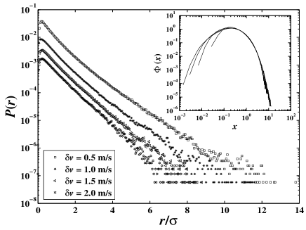
Figure 1: Empirical probability density function $P({r})$ as a function of normalized exit distance ${r}/\sigma$ for $\delta v=0.5$, $1.0$, $1.5$, and $2.0$ m/s. The inset shows the dependence of the corresponding $\Phi(x)$ with respect to $x=r/\sigma$ defined by (3).

Figure 2 presents the fitted exponents $m$ and the characteristic scales $x_{0}$ as a function of $\delta{v}$. Two regimes are observed.

• For $\delta v\lesssim 1.5$, the exponent $m$ increases approximately linearly with $\delta v$ as $m\approx 0.20\times\delta v+0.63$.

• For $\delta v\gtrsim 1.5$, $m$ is approximately constant with a value compatible with $m=1$ corresponding to pure exponential distributions.

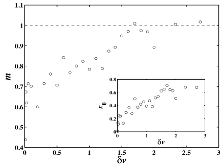
Figure 2: The dependence of the fitted exponents $m$ and characteristic scales $x_{0}$ (inset) with respect to $\delta{v}$.

III.2 Convergence of ${x}^{p}\Phi(x)$

A preliminary condition for analyzing the inverse structure functions is the accuracy of the moments of exit distances. One necessary condition for $T_{p}$ defined by (1) to converge is that the integrand ${r}^{p}P(r)$ or $x^{p}\Phi(x)$ converges to zero at large ${r}$, which requires the closure of the integrand L’vov et al. (1998). We have investigated $x^{p}\Phi(x)$ for different powers $p$ and values $\delta{v}\in[0.01,2.7144]$ to determine how noisy is the range of $r$’s that contribute primarily to $T_{p}(\delta v)$. Fixing $p$, $x^{p}\Phi(x)$ is more noisy for larger $\delta{v}$. For instance, $x^{6}\Phi(x)$ clearly converges for $\delta{v}=0.5$m/s, but not for $\delta{v}=2.0$ m/s. We find that $T_{p}(\delta v)$ with $p$ up to $5$ can be evaluated with good statistical confidence. For $p=6$, a reasonably good evaluation of $T_{6}(\delta v)$ is obtained for small $\delta{v}$. The integrands for $q\geq 8$ seem divergent and the evaluation of the corresponding $T_{p}(\delta{v})$ are less sound statistically. The typical dependence of $x^{p}\Phi(x)$ as a function of $x$ are shown in Fig. 3 for $\delta v=1.5$ m/s and $p=1,2,4,6,8$ and $10$.

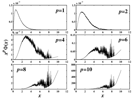
Figure 3: Plots of ${x}^{p}\Phi({x})$ as a function of ${x}$ for different values of $p$ and velocity threshold $\delta v=1.5$ m/s.

We now offer an estimate of the data size needed to estimate reliable inverse structure functions $T_{p}$ for different orders $p$. Let us assume that ${x}$ has a stretched exponential distribution (3) for ${x}$ greater than some ${x}_{0}$. Thus, the integrand of $T_{p}$ is ${\mathcal{I}}(x)=Ax^{p}~{}e^{-(x/x_{0})^{m}}$, where is a normalizing constant. We estimate that a reliable estimation of $T_{p}$ requires a good convergence of the integrant up to a value several times the value $x_{c}$ for which the integrand achieves its maximum (we use a factor $\kappa\approx 2-3$ according to Fig. 3). For the form of the stretched exponential distribution (4), we have ${x}_{c}=x_{0}(p/m)^{1/m}$. On the other hand, the largest typical value $x_{\rm max}$ observed in a sample of size $N$ is determined by the standard condition

$$N\int_{{r}_{\max}}^{\infty}\Phi(x)dx\simeq 1,$$ (5)

where the integration can be performed analytically in terms of a Whittaker $M$ function. When $\Phi(x)$ is exponential, expression (5) leads to the simple equation

$$N=(m/A)e^{m{x}_{\rm max}}~{}.$$ (6)

We now write that $T_{p}(\delta{v})$ is reasonably well-estimated if the range of $x$ extends at least $\kappa$ times beyond $x_{c}$. This amounts to the condition ${x}_{\rm max}=\kappa{x}_{c}$, where $\kappa$ is approximately independent of $\delta{v}$. It follows that the minimum sample size necessary to calculate $T_{p}(\delta{v})$ for an exponential distribution of $x$’s ($m=1$) is given by

$$N(p)=(m/A)e^{\kappa p}~{}.$$ (7)

For $\kappa\simeq 2$ as suggested from the left-middle panels of Fig. 3, with $A\approx 1/x_{0}$ with $x_{0}\approx 0.7$ (see Fig. 2), we find $N(p=8)\approx 6\cdot 10^{6}$ and $N(p=9)\approx 5\cdot 10^{7}$. Thus, our data set with $N\approx 1.7\times 10^{7}$ data points should allow us to get a reasonable estimate of the $8$th order structure function but higher-orders become unreliable.

III.3 Extended self-similarity of inverse structure functions

To investigate the scaling properties of the inverse structure functions, we define a set of relative exponents using the framework of extended self-similarity (ESS) Benzi et al. (1993):

$$T_{p}(\delta v)\propto[T_{p_{0}}(\delta v)]^{\xi(p,p_{0})},$$ (8)

where $p_{0}$ is a reference order. In the case of velocity structure functions, $p_{0}=3$ is a quite natural choice based on the exact Kolmogorov’s four-fifth law. There is no similar reference for the scaling properties of the inverse structure functions and we choose somewhat arbitrarily $p_{0}=2$. In general, ESS provides a wider scaling range for the extraction of scaling exponents. We will see in this subsection that Eq. (8) holds for our experimental data of turbulence with a high accuracy.

Figure 4 presents log-log plots of $T_{p}(\delta v)$ vs $T_{2}(\delta v)$ for $p=1,2,\cdots,10$ with $\delta{v}\in[0.01,2.7144]$. The straight lines hold for $0.2\leq\delta v\leq 2.7144$ and over at least four orders of magnitudes in $T_{2}(\delta v)$, showing the existence of extended self-similarity in the inverse structure functions. The scaling range for small $p$’s seems to be broader than for large $p$’s.

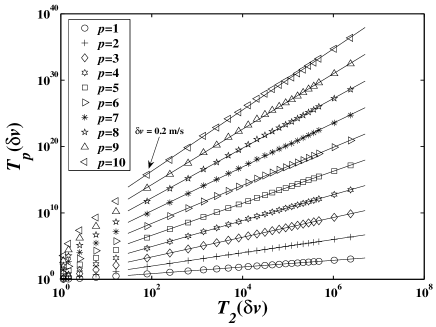
Figure 4: Dependence of the inverse structure function of order $p$ as a function of the inverse structure function of order $2$ taken as a reference. The straight lines exemplify the extended self-similarity of inverse structure functions for the threshold $\delta v$ ranging from $0.2$m/s to $2.7144$m/s.

The ESS scaling exponents $\xi(p,2)$ are shown in Fig. 5. The error bars on $\xi(p,2)$ corresponds to $\pm$ one standard deviation. There is an indication that $\xi(p,2)$ has a nonlinear dependence as a function of $p$, with a downward curvature making the curve depart from the linear dependence $\xi(p,2)=p/2$ observes for small $p$’s.

The monoscaling behavior

$$\xi(p,2)=p/2$$ (9)

is predicted from the assumption that the pdf $\Phi(x)$ of the normalized exit distances, and given by (4), is independent of $\delta v$. By definition, we have $T_{p}(\delta{v})=\langle{{r}^{p}}\rangle_{\delta{v}}=\int_{0}^{\infty}{r}^{p}P_{\delta v}({r})d{r}=[\sigma(\delta v)]^{p}\int_{0}^{\infty}dx~{}\Phi_{\delta v}(x)x^{p}$. Thus,

$$T_{p}(\delta{v})=[T_{2}(\delta{v})]^{p/2}~{}\frac{\int_{0}^{\infty}dx~{}\Phi_{\delta v}(x)~{}x^{p}}{\left[\int_{0}^{\infty}dx~{}\Phi_{\delta v}(x)~{}x^{2}\right]^{p/2}}~{}.$$ (10)

If $\Phi_{\delta v}(x)$ is universal and independent of $\delta v$, then the last term in (10) is a number independent of $\delta v$ (and thus of $T_{2}(\delta{v})$) and the mono-scaling $\xi(p,2)=p/2$ follows. Thus, the prediction (9) holds for those velocity thresholds $\delta{v}$ satisfying the condition that the pdf of exit distance is universal (independent of $\delta v$). This is the analog of the K41 prediction on the standard structure functions. In our present case, there are deviations of the pdf’s of exit distances from the exponential law at small $\delta{v}$, that we have proposed to be quantified under the form of stretched exponentials (4) with exponents $m(\delta v)$ being a function of $\delta v$ as shown in Fig. 2. These deviations from exact self-similarity are weaker than for the direct statistics and are revealed more clearly for the higher orders. We can therefore attribute the deviation of the empirical $\xi(p,2)$ from the self-similarity (9) at high orders to the non-universality of $\Phi_{\delta v}(x)$ which depends on the velocity levels $\delta{v}$.

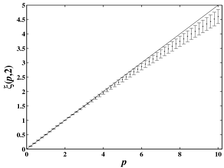
Figure 5: Dependence of the ESS exponents $\xi(p,2)$ as a function of the order $p$ of the inverse structure functions. The straight line is the prediction (9) obtained under the assumption of a universal pdf $\Phi_{\delta v}(x)$ of the exit distances (which is independent of the velocity thresholds $\delta v$).

IV Multifractality of the time series of exit distances at different $\delta{v}$

To investigate further the multifractal nature of the exit distance series $\{r(t):t=1,\cdots,N=3\times 11\times 2^{19}\approx 1.7\times 10^{7}\}$ for a given $\delta{v}$, we construct a probability measure $\mu$ through its integral function $M(t)$

$$\mu\left(]t_{1},t_{2}]\right)=M(t_{2})-M(t_{1})~{},$$ (11)

where $M(t)=0$ for $0<t<1$ and

$$M(t)=\sum_{i=1}^{[t]}r(i)$$ (12)

for $1\leq t\leq N$.

The box-counting method allows us to test for a possible multifractality of the measure $\mu$. The sizes $s$ of the covering boxes are chosen such that the number of boxes of each size is an integer: $n=N/s\in\cal{N}$. We construct the partition function $Z_{q}$ as

$$Z_{q}(s)\triangleq\sum_{i=1}^{n}\left[\mu\left(](i-1)s,is]\right)\right]^{q}~{}.$$ (13)

and expect it to scale as Frisch and Parisi (1985); Halsey et al. (1986)

$$Z_{q}(s)\sim s^{\tau(q)}~{},$$ (14)

which defines the exponent $\tau(q)$. For $\tau(q)$, a hierarchy of generalized dimensions $D_{q}$ Grassberger (1983); Hentschel and Procaccia (1983); Grassberger and Procaccia (1983) can be calculated according to

$$D_{q}=\lim_{p\to q}\frac{\tau(p)}{p-1}~{}.$$ (15)

$D_{0}$ is the fractal dimension of the support of the measure. For our measure (11), we have $D_{0}=1$. The local singularity exponent $\alpha$ of the measure $\mu$ and its spectrum $f(\alpha)$ are related to $\tau(q)$ through a Legendre transformation Halsey et al. (1986)

$$\alpha(q)=d\tau(q)/dq~{},$$ (16a)

and

$$f[\alpha(q)]=q\alpha(q)-\tau(q)~{}.$$ (16b)

We have tested the power-law scaling of $Z_{q}(s)$ as a function of the box size $s$ for the exit time sequences at different velocity levels $\delta{v}$. The scaling range is found to span over four orders of magnitude. Figure 6 plots the partition function $Z_{q}(s)$ for $\delta{v}=1.5$m/s as a function of the box size $s$ for six different values of $q$ in log-log coordinates. The solid lines are the least-square fits with power laws for each $q$. The correlation coefficients of the linear regressions (in log-log) are all larger than $0.997$, demonstrating the existence of a very good scaling.

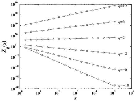
Figure 6: Plots of $Z_{q}(s)$ for $\delta{v}=1.5$m/s as a function of the box size $s$ for different values of $q$ in log-log coordinates. The solid lines are the least-square fits to the data using a linear regression (in log-log coordinates) corresponding to power laws.

The scaling exponents $\tau(q)$ are given by the slopes of the linear fits of $\ln[Z_{q}(s)]$ as a function of $\ln s$ for different values of $\delta{v}$. Figure 7 plots $\tau(q)$ as a function of $q$ for five different velocity levels $\delta v$. The inset shows the fractal spectra $f(\alpha)$ obtained by the Legendre transformation of $\tau(q)$ defined by (16b). We observe that $\tau(q)$’s are concave and nonlinear, a diagnostic of multifractality. The maximal and minimal strength of the set of singularities, $\alpha_{\max}$ and $\alpha_{\min}$, can be approximated asymptotically by $\lim_{q\to\infty}D_{q}=\lim_{q\to\infty}\tau(q)/q$ and $\lim_{q\to-\infty}D_{q}=\lim_{q\to-\infty}\tau(q)/q$, respectively. It can be clearly observed that the steepness of the curve $\tau(q)$ for negative $q$ increases with $\delta{v}$. Consequently, the maximal singularity $\alpha_{\max}$ increases with $\delta{v}$, as shown in the inset of Fig. 7 where the value of $\alpha$ at the right endpoint increases with $\delta{v}$.

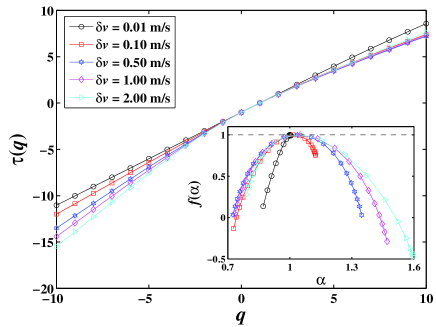
Figure 7: (Color online) Scaling exponents $\tau(q)$ as a function of $q$ for different velocity levels $\delta v$. The inset shows the fractal spectra $f(\alpha)$ obtained by the Legendre transform of $\tau(q)$.

Since $\mu$ is conservative, $\tau(1)=0$ and $\tau(0)=-1$ for all $\delta{v}$. For a given $q<-1$, the function $\tau(q)$ decreases with $\delta{v}$. For a given $q>1$, there is a critical value $\delta{v_{c}}$ such that $d\tau(q)/d\delta{v}<0$ when $\delta{v}<\delta{v_{c}}$ and $d\tau(q)/d\delta{v}>0$ when $\delta{v}>\delta{v_{c}}$. We find that $\delta{v}_{c}$ can be approximated by a linear function

$$\delta{v}_{c}=-0.058q+0.783~{},$$ (17)

associated with a correlation coefficient of the linear regression equal to $0.963$. In addition, one can also see that $\alpha_{\min}$ decreases with $\delta v$ for $\delta{v}<\delta{v_{c}}$ and increases with $\delta v$ for $\delta{v}>\delta{v_{c}}$. For $q=-1$, we find for instance that $\delta{v_{c}}\approx 1.2\rm{m}/\rm{s}$.

We have performed exactly the same multifractal analysis as done above on synthetic time series generated from a stretched exponential distribution and on reshuffled data of the real exit distances. Both tests give linear scaling exponents $\tau(q)=q-1$ in a narrower scaling range $64\leq s\leq 131072$, which is the earmark of monofractality. These tests strengthen the presence of multifractality extracted from the real exit distance data.

In general, multifractality in time series can be attributed to either a hierarchy of changing broad probability density functions for the values of the time series at different scales and/or different long-range temporal correlations of the small and large fluctuations Kantelhardt et al. (2002). Our comparison, with reshuffled data and sequences with the same pdf’s but no correlation which exhibit trivial monofractality, suggests that multifractality in the set of exit distances may be attributed at least in part to the existence non-trivial dependence in the time series of exit distances.

An important feature of the multifractal spectrum $f(\alpha)$ in the inset of Fig. 7 is the existence of negative (or latent) dimensions, that is, $f(\alpha)<0$ Mandelbrot (1989, 1990, 1991); Chhabra and Sreenivasan (1991). The source of negative dimensions could be twofold. Firstly, the turbulent flow is a stochastic process, which introduces intrinsic randomness in the multifractal measure $\mu$. We note that negative dimensions also appear in continuous multifractals Zhou et al. (2001); Zhou and Yu (2001a, b). Secondly, negative dimensions may be interpreted geometrically by considering cuts of higher dimensional multifractals Mandelbrot (1989, 1990, 1991). This intuition proposed by Mandelbrot has been proved mathematically in the multifractal slice theorem Olsen (1998, 1999, 2000). In the present case, the frozen field hypothesis is applied and we deal with one-dimensional cut of the three dimensional turbulence velocity field.

V Concluding remarks

Based on Taylor’s frozen field hypothesis, the statistical properties of the exit distances of 3D turbulence have been investigated. The probability density functions of exit distances at different velocity thresholds have been shown to be well approximated by stretched exponentials. The inverse structure functions was shown to exhibit very clear extended self-similarity (ESS). The ESS exponents $\xi(p,2)$ for small $p<3.5$ are well described by the monofractal prediction $\xi(p,2)=p/2$ obtained by assuming a universal exponential distribution of the exit distance. The multifractality is thus related to the dependence of the pdf’s of the normalized exit distances on the velocity thresholds $\delta v$. We have demonstrated that the sequences of exit distances for each velocity threshold $\delta{v}$ exhibit a clear multifractality with negative dimensions. The scaling ranges over which multifractality holds cover more than four order of magnitude in the exit distance variable. The comparison, with reshuffled data and sequences with the same pdf’s but no correlation which exhibit trivial monofractality, suggests strongly that our report of multifractality is not artifactual.

Our report of multifractality in the time series of exit distance, which tends to emphasize the least turbulent/most laminar regions, suggests a much richer organization of the weakly turbulent and close to laminar regions than believed until recently.