Pricing options with VG model using FFT

Summary

We discuss various analytic and numerical methods that have been used to get option prices within a framework of the VG model. We show that some popular methods, for instance, Carr-Madan’s FFT method [1] could blow up for certain values of the model parameters even for an European vanilla option. Alternative methods - one originally proposed by Lewis, and Black-Scholes-wise method are considered that seem to work fine for any value of the VG parameters. Test examples are given to demonstrate efficiency of these methods. Convergency of all methods is also discussed.

Rutgers University, New Jersey,
Department of mathematics
aitkin@math.rutgers.edu

1 Introduction

This paper summarizes some results of work originally initiated by Peter Carr. It supposes to investigate various numerical and analytical methods of option pricing using VG model in order to find out which algorithm is most efficient.

Let us first give a brief overview of the VG model. The Variance Gamma (VG for short) process was proposed by Madan and Seneta (see [MadanSeneta1990]) to describe stock price dynamics instead of the Brownian motion in the original Black-Scholes model. Two new parameters: $\theta$ skewness and $\nu$ kurtosis are introduced in order to describe asymmetry and fat tails of real life distributions. The VG process is defined by evaluating Brownian motion with drift at a random time specified by gamma process. In other words, the VG model with parameter vector $(\sigma,\nu,\theta)$ assumes that the forward price satisfies the following equation

$$\ln F_{t}=\ln F_{0}+X_{t}+\omega t,$$ (1)

where

$$X_{t}=\theta\gamma_{t}(1,\nu)+\sigma W_{\gamma_{t}(1,\nu)},$$ (2)

and $\gamma_{t}(1,\nu)$ is a Gamma process playing the role of time in this case with unit mean rate and density function given by

$$f_{\gamma_{t}(1,\nu)}(x)=\frac{x^{\frac{t}{\nu}-1}e^{-\frac{x}{\nu}}}{\nu^{\frac{t}{\nu}}\Gamma\left(\frac{t}{\nu}\right)}.$$ (3)

In the Eq. (1) $\omega$ is chosen to make $F_{t}$ a martingale.

The probability density function for the VG process may be written as

$$h_{t}(x)=\int_{0}^{\infty}\frac{\displaystyle dg}{\displaystyle\sqrt{2\pi g}}\exp\left[-\frac{\displaystyle(x-\theta g)^{2}}{\displaystyle 2\sigma^{2}g}\right]\frac{g^{\frac{t}{\nu}-1}e^{-\frac{g}{\nu}}}{\nu^{\frac{t}{\nu}}\Gamma\left(\frac{t}{\nu}\right)}$$ (4)

or after integration over $g$

$$h_{t}(x)=\frac{\displaystyle 2\exp\left(\theta x/\sigma^{2}\right)}{\displaystyle\sqrt{2}\pi\sigma\nu^{\frac{t}{\nu}}\Gamma\left(\frac{t}{\nu}\right)}\left(\frac{\displaystyle x^{2}}{\displaystyle\theta^{2}+\frac{2\sigma^{2}}{\nu}}\right)^{\frac{t}{2\nu}-\frac{1}{4}}K_{\frac{t}{\nu}-\frac{1}{2}}\left(\frac{\displaystyle 1}{\displaystyle\sigma^{2}}\sqrt{x^{2}\left(\theta^{2}+\frac{2\sigma^{2}}{\nu}\right)}\right),$$ (5)

where $K$ is the modified Bessel function of the second kind. The characteristic function $\phi_{\gamma_{t}(1,\nu)}(u)$ for the VG process has remarkably simple form

$$\phi_{t}(u)\equiv\left<E^{iux}\right>\equiv\int_{0}^{\infty}h_{t}(x)e^{iux}dx=\frac{\displaystyle 1}{\displaystyle(1-i\theta\nu u+\frac{1}{2}\sigma^{2}\nu u^{2})^{\frac{t}{\nu}}}.$$ (6)

Another derivation of this expression could be obtained when conditioning on time change like in Romano-Touzi for stochastic volatility models

$$\phi_{\gamma_{t}(1,\nu)}(u) = {\mathbb{E}}[e^{iu\gamma_{t}(1,\nu)}]=\int_{0}^{\infty}e^{iux}f_{\gamma_{t}(1,\nu)}(x)dx=\int_{0}^{\infty}e^{iux}\frac{x^{\frac{t}{\nu}-1}e^{-\frac{x}{\nu}}}{\nu^{\frac{t}{\nu}}\Gamma\left(\frac{t}{\nu}\right)}dx$$ (7)

$$= \int_{0}^{\infty}\frac{x^{\frac{t}{\nu}-1}e^{-\frac{x(1-iu\nu)}{\nu}}}{\nu^{\frac{t}{\nu}}\Gamma\left(\frac{t}{\nu}\right)}dx$$

$$= (1-iu\nu)^{-\frac{t}{\nu}}\int_{0}^{\infty}\frac{(x(1-iu\nu))^{\frac{t}{\nu}-1}e^{-\frac{x(1-iu\nu)}{\nu}}}{\nu^{\frac{t}{\nu}}\Gamma\left(\frac{t}{\nu}\right)}d(x(1-iu\nu))$$

$$= (1-iu\nu)^{-\frac{t}{\nu}}\int_{0}^{\infty}\frac{y^{\frac{t}{\nu}-1}e^{-\frac{y}{\nu}}}{\nu^{\frac{t}{\nu}}\Gamma\left(\frac{t}{\nu}\right)}dy=(1-iu\nu)^{-\frac{t}{\nu}}.$$

$$\phi_{X_{t}}(u) = {\mathbb{E}}[e^{iuX_{t}}]={\mathbb{E}}[{\mathbb{E}}[e^{iuX_{t}}\mid\gamma_{t}(1,\nu)]]={\mathbb{E}}[{\mathbb{E}}[e^{iu\left(\theta\gamma_{t}(1,\nu)+\sigma W_{\gamma_{t}(1,\nu)}\right)}\mid\gamma_{t}(1,\nu)]]$$ (8)

$$= {\mathbb{E}}[e^{iu\theta\gamma_{t}(1,\nu)-\frac{1}{2}u^{2}\sigma^{2}\gamma_{t}(1,\nu)}]={\mathbb{E}}[e^{i\left(u\theta+i\frac{1}{2}u^{2}\sigma^{2}\right)\gamma_{t}(1,\nu)}]$$

$$= \phi_{\gamma_{t}(1,\nu)}(u\theta+i\frac{1}{2}u^{2}\sigma^{2})=\left(1-i\theta\nu u+\frac{1}{2}\sigma^{2}\nu u^{2}\right)^{-\frac{t}{\nu}}.$$

Now, to prevent arbitrage, we need $F_{t}$ be a martingale, and, since $F_{t}$ is already an independent increment process, all we need is

$${\mathbb{E}}[F_{t}]=F_{0},$$ (9)

or

$${\mathbb{E}}[F_{0}e^{X_{t}+\omega t}]=F_{0}\phi_{X_{t}}(-i)e^{\omega t}=F_{0}.$$ (10)

This tells us that

$$\omega=-\frac{\ln\phi_{X_{t}}(-i)}{t}=-\frac{-\frac{t}{\nu}\ln\left(1-\theta\nu-\frac{1}{2}\sigma^{2}\nu\right)}{t}=\frac{1}{\nu}\ln\left(1-\theta\nu-\frac{1}{2}\sigma^{2}\nu\right).$$ (11)

Note that from the definition of $\omega$ above, in order to have a risk neutral measure for VG model, its parameters must obey an inequality:

$$\frac{\displaystyle 1}{\displaystyle\nu}>\theta+\frac{\sigma^{2}}{2}.$$ (12)

Note that risk neutral parameters $\theta,\nu,\sigma$ do not have to be equal to their statistical counterparts.

Accordingly, the characteristic function of the $x_{T}\equiv\log S_{T}$ VG process is

$$\phi(u)=\frac{\displaystyle S_{0}e^{(r-q+\omega)T}}{\displaystyle\left(1-i\theta\nu u+\frac{1}{2}\sigma^{2}\nu u^{2}\right)^{\frac{T}{\nu}}}.$$ (13)

Statistical parameters of VG distribution may be calculated from the historical data on stock prices. In particular we have to find the values of the parameters $\theta^{*},\nu^{*}$ and $\sigma^{*}$ such that the folloiwng expression is maximized:

$$\prod_{j=1}^{n}h_{\tau_{j}}(x_{j}),$$ (14)

where $h_{\tau_{j}}(x_{j})$ are given by Eq.5 and $x_{j}$ are observed returns per time $\tau_{j}$, i.e. $x_{j}=\log(S_{j}/S_{j-1})$.

2 Pricing European option

The value of European option on a stock when the risk neutral dynamics is given by Eq. (1) is

$$V=\exp(-rT)\int_{-\infty}^{\infty}h_{T}\left(x-(r-q+\omega)T\right)W(e^{x})dx,$$ (15)

where $T$ is time until expiration, $q$ is continuous dividend and $W(e^{x})$ is payoff function that has the following form

$$W(e^{x})=(S_{0}e^{x}-K)^{+}-\mbox{call},\quad W(e^{x})=(K-S_{0}e^{x})^{+}-\mbox{put}.$$ (16)

Direct calculation allows us to derive the put-call parity relation identical to Black-Scholes case

$$C=S_{0}e^{-qT}-Ke^{-rT}+P.$$ (17)

There are several methods to price a European option under the VG model. One method uses the closed form solution derived in [2]. Although the expression is analytic it requires computation of modified Bessel functions, and hence may not be as fast as we would like our pricing model to be. Therefore, FFT method has been widely utilized to obtain a more efficient pricer. Few flavors of the FFT method has been previously discussed with regard to the VG model.

First of all the FFT method of Carr and Madan [1], nowadays almost standard in math finance, was applied to the VG model to price the European vanilla option since the characteristic function of the log-return process has a very simple form given above. Further we intend to show, that unfortunately this method blows up at some values of the VG parameters.

Mike Konikov and Dilip Madan [3] proposed another interesting method based on the definition of the VG process as being a time changed Brownian motion, where the time change is assumed independent of the Brownian motion. This method was described in detail in [3] while has not been implemented yet.

Also Mike Konikov and I independently implemented a modification of the FFT method - the Fractional Fourier Transform, which is described in detail in [4, 5]. This method usually allows acceleration of the pricing function by factor 8-10, while for the VG model it still demonstrates same problem as the original FFT.

Below we discuss why the Carr and Madan FFT approach fails for the VG model. We propose another method, which originally has been developed in a general form by Lewis [6], that seems to be free of such problems.

3 Carr-Madan’s FFT approach and the VG model

Let us start with a short description of the Carr-Madan FFT method. It was worked out for models where the characteristic function of underlying price process ($S_{t}$) is available. Therefore, the vanilla options can be priced very efficiently using FFT as described in Carr and Madan  [1]. The characteristic function of the price process is given by

$$\phi(u,t)={\mathbb{E}}(e^{iuX_{t}}),$$ (18)

where $X_{t}=\log(S_{t})$. Note that the above representation holds for all models and is not just restricted to Lévy models where the characteristic functions have a time homogeneity constraint that $\phi(u,t)=e^{-t\psi(u)}$, where $\psi(u)$ is the Lévy characteristic exponent.

Once the characteristic function is available, then the vanilla call option can be priced using Carr-Madan’s FFT formula:

$$C(K,T)=\frac{e^{-\alpha\log(K)}}{\pi}\int_{0}^{\infty}\mathrm{Re}\left[e^{-iv\log(K)}\omega(v)\right]dv,$$ (19)

where

$$\omega(v)=\frac{e^{-rT}\phi(v-(\alpha+1)i,T)}{\alpha^{2}+\alpha-v^{2}+i(2\alpha+1)v}$$ (20)

The integral in the first equation can be computed using FFT, and as a result we get call option prices for a variety of strikes. For complete details, see Carr & Madan paper [1].

The put option values can just be constructed from Put-Call symmetry.

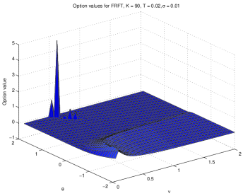
Figure 1: European option values in VG model at $T=0.02yrs,K=90,\sigma=0.01$ obtained with FRFT.

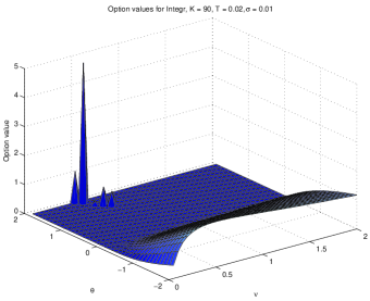
Figure 2: European option values in VG model at $T=0.02yrs,K=90,\sigma=0.01$ obtained with the adaptive integration.

Parameter $\alpha$ in Eq. (19) must be positive. Usually $\alpha=3$ works well for various models. It is important that the denominator in Eq. (20) has only imaginary roots while integration in Eq. (19) is provided along real $v$. Thus, the integrand of Eq. (19) is well-behaved.

But as it turned out, this is not the case for the VG model. To show this let us consider the European call option values obtained by Mike Konikov by computing FFT of the VG characteristic function according to Eq. (19).

In Fig. 2 the results of that test obtained using the FRFT algorithm are given for strike $K=90$, maturity $T=0.02$ yrs and volatility $\sigma=0.01$. It is seen that at positive coefficients of skew $\Theta\approx 2$ and coefficients of kurtosis $\nu\approx 0.5$ the option value has a delta-function-wise pick that doesn’t seem to be a real option value behavior. In Fig. 2 similar results are obtained using a different method of evaluation of the integral in Eq. (19) - an adaptive integration. Eventually, in Fig. 4 same test was provided using a standard FFT method. The results look quite different that allows a guess that something is wrong with FRFT and the adaptive integration. One could also note that this test plays with an option with a very short maturity. Therefore, to let us make another test with a longer maturity. In Fig. 4-6 the results of the test that uses same integration procedures, but for the option with $K=90,T=1,\sigma=1$, are presented. It is seen that for longer maturities FFT also blows up almost at the same region of the model parameters. Moreover, it occurs not only at positive value of the skew coefficient but at negative as well. Thus, the problem lies not in the numerical method that was used to evaluate the integral in the Eq. (19), but in the integral itself.

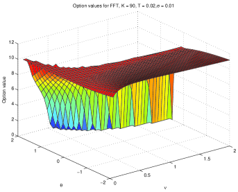
Figure 3: European option values in VG model at $T=0.02yrs,K=90,\sigma=0.01$ obtained with FFT.

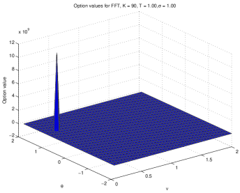
Figure 4: European option values in VG model at $T=1.0yrs,K=90,\sigma=1.0$ obtained with the FFT.

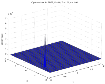
Figure 5: European option values in VG model at $T=1.0yrs,K=90,\sigma=1.0$ obtained with the FRFT.

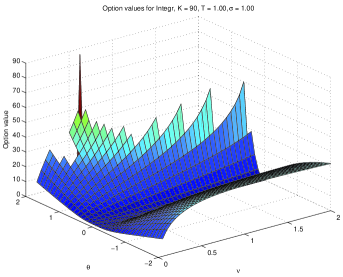
Figure 6: European option values in VG model at $T=1.0yrs,K=90,\sigma=1.0$ obtained with the adaptive integration.

Now having expression Eq. (6) for the VG characteristic function let us substitute it and Eq. (20) into the Eq. (19) that gives

$$C(K,T)\propto\frac{\displaystyle e^{-\alpha\log(K)-rT}}{\displaystyle\pi}\int_{0}^{\infty}\Re\left\{\frac{\displaystyle e^{-iv\log(K)}}{\displaystyle\left[\alpha^{2}+\alpha-v^{2}+i(2\alpha+1)v\right]\left(1-i\theta\nu u+\frac{1}{2}\sigma^{2}\nu u^{2}\right)^{\frac{t}{\nu}}}\right\}dv,$$ (21)

where $u\equiv v-(\alpha+1)i$. At small $T$ close to zero the second term in the denominator of the Eq. (21) is close to 1. Therefore at small $T$ the denominator has no real roots. To understand what happens at larger maturities, let us put $T=0.8,\nu=0.1,\alpha=3,\sigma=1$ and see how the denominator behaves as a function of $v$ and $\Theta$. The results of this test obtained with the help of Mathematica package are given in Fig 8.

It is seen that at $v=0$ at positive $\Theta$ the characteristic function has a singularity. To investigate it in more detail, we assume $v=0$ and plot the denominator as a function of $\sigma$ and $\Theta$ (see Fig. 8). As follows from this Figure in the interval $0<\sigma<2$ there exists a value of $\Theta$ that makes the integrand in the Eq. (21) singular. This means that singularity of the integrand can not be eliminated, and thus the Carr-Madan FFT method can not be used together with the VG model for pricing European vanilla options. Using FRFT or adaptive integration that both are slight modifications of the FFT, also doesn’t help.

Note that for the VG model the authors of [1] derived condition which keeps the characteristic function to be finite, that reads

$$\alpha<\sqrt{\frac{\displaystyle 2}{\displaystyle\nu\sigma^{2}}+\frac{\displaystyle\Theta^{2}}{\displaystyle\sigma^{4}}}-\frac{\displaystyle\Theta}{\displaystyle\sigma^{2}}-1.$$ (22)

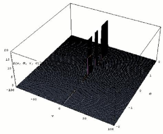
Figure 7: Denominator of the Eq. (21) at $T=0.8,\nu=0.1,\alpha=3,\sigma=1$ as a function of $v$ and $\Theta$.

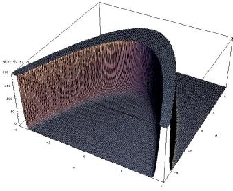
Figure 8: Denominator of the Eq. (21) at $T=0.8,\nu=0.1,\alpha=3,v=0$ as a function of $\sigma$ and $\Theta$.

Also as can be seen, for $\Theta,\nu$ and $\sigma$ corresponding to the above mentioned tests $\alpha$ becomes negative that doesn’t allow using this method to price the options in terms of strike.

In order to solve these problems one needs to find another way how to regularize the integrand, i.e. eliminate doing it in the way as Carr and Madan did it using a regularization factor $e^{-\alpha k}$.

4 Lewis’s regularization

Another approach of how to apply FFT to the pricing of European options was proposed by Alan Lewis [6]. Lewis notes that a general integral representation of the European call option value with a vanilla payoff is

$$C_{T}(x_{0},K)=e^{-rT}\int_{-\infty}^{\infty}\left(e^{x}-K\right)^{+}q(x,x_{0},T)dx,$$ (23)

where $x=\log S_{T}$ is a stock price that under a pricing measure evolves as $S_{T}=S_{0}\exp[(r-q)T+X_{T}$, $r-q$ is the cost of carry, $T$ is the expiration time for some option, $X_{T}$ is some Levy process satisfying ${\mathbb{E}}[exp(iuX_{T})]=1$, and $q$ is the density of the log-return distribution $x$.

The central point of the Lewis’s work is to represent the Eq. (23) as a convolution integral and then apply a Parseval identity

$$\int_{-\infty}^{\infty}f(x)g(x_{0}-x)dx=\frac{\displaystyle 1}{\displaystyle 2\pi}\int_{-\infty}^{\infty}e^{-iux_{0}}\hat{f}(u)\hat{g}(u)du,$$ (24)

where the hat over function denotes its Fourier transform.

The idea behind this formula is that the Fourier transform of a transition probability density for a Levy process to reach $X_{t}=x$ after the elapse of time $t$ is a well-known characteristic function, which plays an important role in mathematical finance. For Levy processes it is $\phi_{t}(u)={\mathbb{E}}[\exp(iuX_{t})],u\in\Re$, and typically has an analytic extension (a generalized Fourier transform) $u\rightarrow z\in{\mathbb{C}}$, regular in some strip ${\cal S}_{X}$ parallel to the real z-axis.

Now suppose that the generalized Fourier transform of the payoff function $\hat{w}(z)=\int_{-\infty}^{\infty}e^{izx}(e^{x}-K)^{+}dx$ and the characteristic function $\phi_{t}(z)$ both exist (we will discuss this below). Then from a chain of equalities the call option value can be expressed as follows

$$C_{T}(x_{0},K) = e^{-rT}{\mathbb{E}}\left[\left(e^{x}-K\right)^{+}\right]=\frac{\displaystyle e^{-rT}}{\displaystyle 2\pi}{\mathbb{E}}\left[\int_{i\mu-\infty}^{i\mu+\infty}e^{-izx_{T}}\hat{w}(z)dz\right]$$

$$= \frac{\displaystyle e^{-rT}}{\displaystyle 2\pi}{\mathbb{E}}\left[\int_{i\mu-\infty}^{i\mu+\infty}e^{-iz[x_{0}+(r-q+\omega)T]}e^{-izX_{T}}\hat{w}(z)dz\right]$$

$$= \frac{\displaystyle e^{-rT}}{\displaystyle 2\pi}\int_{i\mu-\infty}^{i\mu+\infty}e^{-iz[x_{0}+(r-q+\omega)T]}{\mathbb{E}}[e^{-izX_{T}}]\hat{w}(z)dz=\frac{\displaystyle e^{-rT}}{\displaystyle 2\pi}\int_{i\mu-\infty}^{i\mu+\infty}e^{-izY}\phi_{X_{T}}(-z)\hat{w}(z)dz.$$

Here $Y=x_{0}+(r-q+\omega)T$, $\mu\equiv$ Im $z$. This is a formal derivation which becomes a valid proof if all the integrals in Eq. (4) exist.

The Fourier transform of the vanilla payoff can be easily found by a direct integration

$$\hat{w}(z)=\int_{-\infty}^{\infty}e^{izx}(e^{x}-K)^{+}dx=-\frac{\displaystyle K^{iz+1}}{\displaystyle z^{2}-iz},\qquad\mathrm{Im}z>1.$$ (26)

Note that if z were real, this regular Fourier transform would not exist. As shown in [7], payoff transforms $\hat{w}(z)$ for typical claims exist and are regular in their own strips ${\cal S}_{w}$ in the complex z-plane, just like characteristic functions.

Above we denoted the strip where the characteristic function $\phi(z)$ is well-behaved as ${\cal S}_{X}$. Therefore, $\phi(-z)$ is defined at the conjugate strip ${\cal S}^{*}_{X}$. Thus, the Eq. (4) is defined at the strip ${\cal S}_{V}={\cal S}^{*}_{X}\bigcap{\cal S}_{w}$, where it has the form

$$C(S,K,T)=-\frac{\displaystyle Ke^{-rT}}{\displaystyle 2\pi}\int_{i\mu-\infty}^{i\mu+\infty}e^{-izk}\phi_{X_{T}}(-z)\frac{\displaystyle dz}{\displaystyle z^{2}-iz},\quad\mu\in{\cal S}_{V},$$ (27)

and $k=\log(S/K)+(r-q+\omega)T$.

The characteristic function of the VG process has been given by the Eq. (13) and is defined in the strip $\beta-\gamma<$ Im $z<\beta+\gamma$, where

$$\beta=\frac{\displaystyle\Theta}{\displaystyle\sigma^{2}},\quad\gamma=\sqrt{\frac{\displaystyle 2}{\displaystyle\nu\sigma^{2}}+\frac{\displaystyle\Theta^{2}}{\displaystyle\sigma^{4}}+2(\mathrm{Re}z)^{2}}.$$ (28)

This condition can be relaxed by assuming in the Eq. (28) $\mathrm{Re}z=0$ . Accordingly, $\phi(-z)$ is defined in the strip $\gamma-\beta>$ Im $z>-\beta-\gamma$.

Now let us choose Im $z$ in the form

$$\mu\equiv\mathrm{Im}\ z=\sqrt{1+\frac{\displaystyle 2\Theta}{\displaystyle\sigma^{2}}+\frac{\displaystyle\Theta^{2}}{\displaystyle\sigma^{4}}}-\frac{\displaystyle\Theta}{\displaystyle\sigma^{2}}.$$ (29)

Taking into account the Eq. (12) which makes a constrain on the available values of the VG parameters, it is easy to see that $\mu$ defined in such a way obeys the inequality $\mu<\gamma-\beta$. On the other hand, as also can be easily seen, $\mu\geq 1$ at any value of $\Theta$ and positive volatilities $\sigma$, and the equality is reached when $\Theta=0$. It means, that Im $z=\mu$ lies in the strip ${\cal S}^{*}_{X}$ as well as in the strip ${\cal S}_{w}$, i. e. $\mu\in{\cal S}_{V}$.

Now one more trick with contour integration. The integrand in Eq. (27) is regular throughout ${\cal S}^{*}_{X}$ except for simple poles at $z=0$ and $z=i$. The pole at $z=0$ has a residue $-Ke^{-rT}i/(2\pi)$, and the pole at $z=i$ has a residue $Se^{-qT}i/(2\pi)$ . The analysis of the previous paragraph shows that the strip ${\cal S}^{*}_{X}$ is defined by the condition $\gamma-\beta>\mathrm{Im}z>-\beta-\gamma$, where $\gamma-\beta>1$, and $-\beta-\gamma<0$. Therefore we can move the integration contour to $\mu_{1}\in(0,1)$. Then by the residue theorem, the call option value must also equal the integral along Im $z=\mu_{1}$ minus $2\pi i$ times the residue at $z=i$. That gives us a first alternative formula

$$C(S,K,T)=Se^{-qT}-\frac{\displaystyle Ke^{-rT}}{\displaystyle 2\pi}\int_{i\mu_{1}-\infty}^{i\mu_{1}+\infty}e^{-izk}\phi_{X_{T}}(-z)\frac{\displaystyle dz}{\displaystyle z^{2}-iz}$$ (30)

For example, with $\mu_{1}=1/2$ which is symmetrically located between the two poles, this last formula becomes

$$C(S,K,T)=Se^{-qT}-\frac{\displaystyle 1}{\displaystyle\pi}\sqrt{SK}e^{-(r+q)T/2}\int_{0}^{\infty}\mathrm{Re}\left[e^{-iu\kappa}\Phi\left(-u-\frac{\displaystyle i}{\displaystyle 2}\right)\right]\frac{\displaystyle du}{\displaystyle u^{2}+\frac{1}{4}}\\$$ (31)

where $\kappa=\ln(S/K)+(r-q)T,\quad\Phi(u)=e^{iu\omega T}\phi_{X_{T}}(u)$ and it is taken into account that the integrand is an even function of its real part. The last integral can be rewritten in the form

$$\int_{0}^{\infty}e^{-iu\ln\kappa}\phi_{1}(u)du,\qquad\phi_{1}(u)=\frac{\displaystyle 4}{\displaystyle 4u^{2}+1}\Phi\left(-u-\frac{\displaystyle i}{\displaystyle 2}\right).$$ (32)

This can be immediately recognized as a standard inverse Fourier transform, and by derivation the integrand is regular everywhere. Indeed, $\phi_{X_{T}}(-u-i/2)|_{u=0}=(1-\frac{\sigma^{2}\nu}{8}-\frac{\nu\theta}{2})^{-t/\nu}$, therefore the denominator vanishes if $\frac{2}{\nu}=\theta+\frac{\sigma^{2}}{4}$. Now using the Eq. (12) one finds that $\theta+\frac{\sigma^{2}}{4}>2h+\sigma^{2}$ or $\frac{\sigma^{2}}{4}<-\frac{\theta}{3}$. Thus, $\theta$ must be negative to turn the denominator to zero. The last equality could be also rewritten as $\theta+\frac{\sigma^{2}}{4}<\frac{2\theta}{3}$. Thus, the denominator vanishes if $\frac{1}{\nu}<\frac{2\theta}{3}$, i.e. $\nu$ must be negative, but it is not! Therefore, the characteristic function in Eq. (32) doesn’t have singularity at $u=0$. Thus, a standard FFT or FRFT method can be applied to get the value of the integral.

In Fig. 11 -11 the results of the European vanilla option pricing with the VG model conducted by using this new FFT method are displayed. Two test has been provided with parameters $T=1$ yr, $K=90,\sigma=0.1$ (Fig. 11) and $T=1$ yr, $K=90,\sigma=0.5$ (Fig. 11). It is seen that the option value surface is regular in both cases. Zero values indicates that region, where the VG constrain Eq. (12) is not respected. The higher values of $\sigma$ and $\Theta$ are the lower values of $\nu$ are required to obey this constraint. Therefore, at higher values of $\nu$ the model is not defined that produces irregularity in the graph. This effect is better observable in Fig. 11 that is obtained by rotation of the Fig. 11. The above means that the new FFT method can be used with no essential problem. A generalization of this method for FRFT is also straightforward.

In the region of the VG parameters values where an application of the Carr-Madan FFT procedure doesn’t cause the problem the results of that method are almost identical to what the described above method gives. An example of such a comparison is given in Fig. 12 (my NewFFT Matlab code vs Mike’s FFT code). It is seen that the difference is of the order of $10^{-7}$.

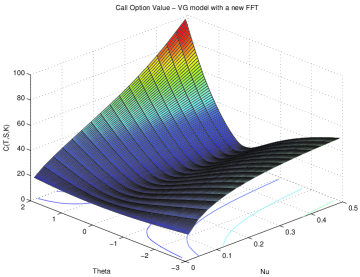
Figure 9: European option values in VG model at $T=1.0yr,K=90,\sigma=0.1$ obtained with the new FFT method.

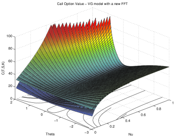
Figure 10: European option values in VG model at $T=1.0yrs,K=90,\sigma=0.5$ obtained with the new FFT method.

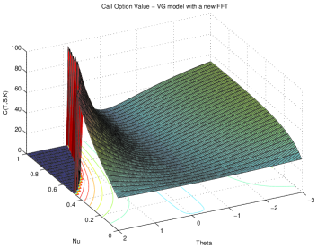
Figure 11: European option values in VG model at $T=1.0yr,K=90,\sigma=0.5$ obtained with the new FFT method (rotated graph).

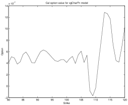
Figure 12: The difference between the European call option values for the VG model obtained with Carr-Madan FFT method and the new FFT method. Parameters of the test are: $S=100,T=0.5yr,\sigma=0.2,\nu=0.1,\Theta=-0.33,r=q=0.$ at various strikes).

5 Black-Scholes-wise method

One more method of regularization of the Fourier kernel for the VG model has been proposed by Sepp [8] and is also discussed in [9], [10]. The idea is as follows.

Given characteristic function $\phi_{X_{t}}(z)$ of the model $M$ the price of a European option can be expressed as

$$\Pi_{1}^{M} = \frac{\displaystyle 1}{\displaystyle 2}+\frac{\displaystyle\xi}{\displaystyle 2\pi}\int_{-\infty}^{\infty}\frac{\displaystyle e^{-iu\ln K}e^{iu[\ln S+(r-q+\omega)T]}\phi_{X_{T}}(u-i)}{\displaystyle iu\phi_{X_{T}}(-i)}du,$$ (33)

$$\Pi_{2}^{M} = \frac{\displaystyle 1}{\displaystyle 2}+\frac{\displaystyle\xi}{\displaystyle 2\pi}\int_{-\infty}^{\infty}\frac{\displaystyle e^{-iu\ln K}e^{iu[\ln S+(r-q+\omega)T]}\phi_{X_{T}}(u)}{\displaystyle iu}du,$$

$$V^{M} = \xi\left[e^{-qT}S_{0}\Pi_{1}^{M}-e^{-rT}K\Pi_{2}^{M}\right],$$

where $\xi=1(-1)$ for a call(put). Eq. (33) is a generalization of the Black-Scholes option pricing formula. Note that $\phi_{X_{t}}(0)=1$ by definition, and $\phi_{X_{t}}(-i)$ is a function of time to expiry $T$ and parameters of the model only.

Proof: Assume that $\phi_{T}(-z)$ has a strip of regularity $0\leq\mu\leq 1$. First we rewrite Eq. (27) as

$$C(S,K,T) = -\frac{\displaystyle Ke^{-rT}}{\displaystyle 2\pi}\int_{i\mu-\infty}^{i\mu+\infty}e^{-izk}\phi_{X_{T}}(-z)\frac{\displaystyle dz}{\displaystyle z^{2}-iz}$$

$$= -\frac{\displaystyle Ke^{-rT}}{\displaystyle 2\pi}\left[\int_{i\mu-\infty}^{i\mu+\infty}e^{-izk}\phi_{X_{T}}(-z)\frac{\displaystyle idz}{\displaystyle z}-\int_{i\mu-\infty}^{i\mu+\infty}e^{-izk}\phi_{X_{T}}(-z)\frac{\displaystyle idz}{\displaystyle z-i}\right]$$

$$= -\frac{\displaystyle Ke^{-rT}}{\displaystyle 2\pi}({\cal R}(I_{1})-{\cal R}(I_{2}))$$

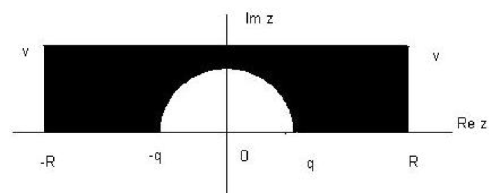
Figure 13: Integration contour for ${\cal R}(I_{1})$

.

In order to evaluate $I_{1}$ we employ a contour integral over the contour given by 6 parametric curves (see Fig. (13): $\Gamma_{1}:z=u,u\in(q,R),q,R>0;\Gamma_{2}:z=R+ib,b\in(0,v);\Gamma_{3}:z=u+iv,u\in(R,-R);\Gamma_{4}:z=-R+ib,b\in(v,0);\Gamma_{5}:z=u,u\in(-R,-q);\Gamma_{6}:z=qe^{i\theta},\theta\in(\pi,0)$. As the integrand is analytic on this contour we can apply the Cauchy theorem. Also note that the integral along curve $\Gamma_{6}$ is a half of the integral along the whole circle around zero which in turn is equal to $2\pi i^{2}Res(e^{-izk}\phi_{t}(-z)/z)$. As the integrals along vertical lines vanish at $R\rightarrow\infty$ and at $q\rightarrow 0$ the integral along the real axis tends to an integral from $-\infty$ to $\infty$, eventually changing variable $u\rightarrow-u$ we obtain

$${\cal R}(I_{1})=\pi+\int_{-\infty}^{\infty}e^{-iu\ln K}e^{iu[\ln S+(r-q+\omega)T]}\frac{\displaystyle\phi_{X_{T}}(u)}{\displaystyle iu}du.$$ (35)

To compute the ${\cal R}(I_{2})$ we use a similar contour build around the point $z=i$, i.e. $\Gamma_{1}:z=u+i,u\in(q,R),q,R>0;\Gamma_{2}:z=R+ib,b\in(1,1+v);\Gamma_{3}:z=u+i(1+v),u\in(R,-R);\Gamma_{4}:z=-R+ib,b\in(v,1);\Gamma_{5}:z=u+i,u\in(-R,-q);\Gamma_{6}:z=i+qe^{i\theta},\theta\in(0,\pi)$. Again taking limits $R\rightarrow\infty$ and $q\rightarrow 0$, changing variable $u\rightarrow u-i$, we obtain

$${\cal R}(I_{2})=\frac{\displaystyle S}{\displaystyle K}e^{(r-q)T}\left(\pi+\int_{-\infty}^{\infty}e^{-iu\ln K}e^{iu[\ln S+(r-q+\omega)T]}\frac{\displaystyle\phi_{X_{T}}(u-i)}{\displaystyle iu\phi_{X_{T}}(-i)}du\right).$$ (36)

Substituting these integrals into the Eq. (5) we obtain the Eq. (33) $\blacksquare$.

The difficulty in using FFT to evaluate the Eqs. (33), as noted by Carr and Madan is the divergence of the integrands at $u=0$. Specifically, let us develop the characteristic function $\phi_{X_{t}}(z)$ with $z=u+iv$ as Taylor series in $u$

$$\phi_{X_{t}}(z)={\mathbb{E}}[e^{-vX_{t}}]+iu{\mathbb{E}}[xe^{-vX_{t}}]-\frac{1}{2}u^{2}{\mathbb{E}}[x^{2}e^{-vX_{t}}]+...$$ (37)

In Eq. (30) we have to chose $z=u-i$ in the first expression, and $z=u$ in the second one. As it is easy to check in both cases that the leading term in the expansion under both integrals is $1/(iu)$ which is just a source of the divergence.The source of this divergence is a discontinuity of the payoff function at $K=S_{T}$. Accordingly the Fourier transform of the payoff function has large high-frequency terms. The Carr-Madan solution is in fact to dampen the weight of the high frequencies by multiplying the payoff by an exponential decay function. This will lower the importance of the singularity, but at the cost of degradation of the solution accuracy.

As the Eqs. (33) can be used whenever the characteristic function of the given model is known, we can apply it to the Black-Scholes model as well that gives us the Black-Scholes option price $V^{BS}$ which is a well known analytic expression. Now the idea is to rewrite representation of the option price in the Eqs. (33) in the form

$$V^{M}=[V^{M}-V^{BS}]+V^{BS}.$$ (38)

The term in braces can now be computed with FFT as

$$\Pi_{1}^{M-BS} = \frac{\displaystyle\xi}{\displaystyle 2\pi}\int_{-\infty}^{\infty}\frac{\displaystyle e^{-iu\kappa}\left[\phi_{X_{t}}(u-i)e^{i(u-i)\omega T}-\phi_{BS}(u-i)e^{-\frac{\sigma^{2}}{2}T}\right]}{\displaystyle iu}du,$$ (39)

$$\Pi_{2}^{M-BS} = \frac{\displaystyle\xi}{\displaystyle 2\pi}\int_{-\infty}^{\infty}\frac{\displaystyle e^{-iu\kappa}\left[\phi_{X_{t}}(u)e^{iu\omega T}-\phi_{BS}(u)\right]}{\displaystyle iu}du,$$

$$V^{M}-V^{BS} = \xi\left[e^{-qT}S_{0}\Pi_{1}^{M-BS}-e^{-rT}K\Pi_{2}^{M-BS}\right],$$

where $\kappa=\ln(K/S)-(r-q)T$, $\phi_{BS}(u)=\exp\left(-\frac{\sigma^{2}T}{2}u^{2}\right)$ and $\phi_{X_{T}}(-i)=e^{-\omega T}$. This is possible because we have removed the divergence in the integrals. In addition the magnitude of $\phi_{X_{t}}(z)-\phi_{BS}(z)$ is smaller than that of $\phi_{X_{t}}(z)$ that increases accuracy of the solution.

In more detail, first terms of the expansion of $\phi_{X_{t}}(u)e^{iu\omega T}-\phi_{BS}(u)$ and $\phi_{X_{t}}(u-i)e^{i(u-i)\omega T}-\phi_{BS}(u-i)e^{-\frac{\sigma^{2}}{2}T}$ in series at small $u$ are

$$D_{1}|_{u=0} \equiv \phi_{X_{t}}(u)e^{iu\omega T}-\phi_{BS}(u)=T(\theta+\omega+\frac{\displaystyle\sigma^{2}}{\displaystyle 2})iu+O(u^{2})$$ (40)

$$D_{2}|_{u=0} \equiv \phi_{X_{t}}(u-i)e^{i(u-i)\omega T}-\phi_{BS}(u-i)e^{-\frac{\sigma^{2}}{2}T}=-\left(\sigma^{2}+\frac{\theta+\sigma^{2}}{-1+\nu(\theta+\sigma^{2}/2)}-\omega\right)iu+O(u^{2})$$

However, an usage of these expressions in the Eq. (39) together with the FFT method produces an error of the order of $O(u)$. That is why it is better to choose a small $u=\epsilon$, for instance $\epsilon=10^{-6}$, then computing integrands in the Eq. (39) exactly and substituting $D_{1,2}|_{u=0}\approx D_{1,2}|_{u=\epsilon}$.

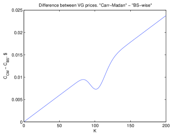
Figure 14: European option values in VG model. Difference between the Carr-Madan solution and Black-Scholes-wise solution with $D_{1,2}(u=0)$ at $T=1.0yr,\sigma=0.1,\theta=0.1,\nu=0.1$

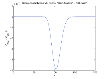
Figure 15: European option values in VG model. Difference between the Carr-Madan solution and Black-Scholes-wise solution with $D_{1,2}(u=\epsilon)$ at $T=1.0yr,\sigma=0.1,\theta=0.1,\nu=0.1$

Fig. 15, 15 show the results of our computation of the European option values under the VG model. Difference between the Carr-Madan solution and Black-Scholes-wise solution with $D_{1,2}(u=\epsilon)$ and $D_{1,2}(u=0)$ at $T=1.0yr,\sigma=0.1,\theta=0.1,\nu=0.1$ are plotted for 200 strikes. It is seen that for the first method the difference is of the order of 0.5%.

6 Convergency and performance

Artur Sepp reported in [8] that the convergency of the Black-Scholes-wise method is approximately 3 times faster than that of the Lewis method. It could be understood because as we mentioned above in the limit of small $u$ the difference between the VG solution and the Black-Scholes formula which is under the Fourier integral is of the second order in $u$ while in the Lewis method it is of the zero order. In other words using the Black-Scholes-wise formula allows us to remove a part of the FFT error instead substituting it with the exact analytical solution of the Black-Scholes problem.

We also fulfilled investigation of how all three methods converge for the VG model. The results are given in Fig. 17,17,19. We display $\log_{10}$ difference between the option price obtained with $N=8192$, and that with $N=4096,1024,512,256$. We don’t see much difference in the convergency of the Lewis and Black-Scholes-wise method while the Carr-Madan methods behaves better at low $N$. In Fig. 19 we also present the ratio $(C_{N=8192}-C_{N=4096})/C_{N=8192}$ for all three methods. The Carr-Madan still converges better for out of the money spot prices while convergency of two other methods is similar.

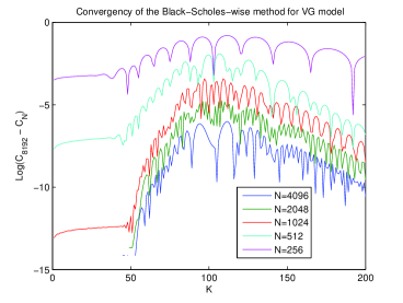
Figure 16: Convergency of the Black-Scholes-wise method. Difference between the option price obtained with $N=8192$, and that with $N=4096,1024,512,256$

.

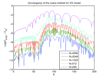
Figure 17: Convergency of the Lewis method. Difference between the option price obtained with $N=8192$, and that with $N=4096,1024,512,256$

.

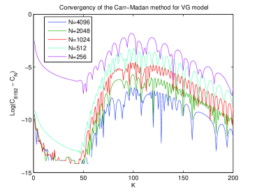
Figure 18: Convergency of the Carr-Madan method. Difference between the option price obtained with $N=8192$, and that with $N=4096,1024,512,256$

.

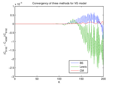
Figure 19: Convergency of all three methods

.

Cont and Tankov also analyze the Lewis method. They emphasize the fact that the integral in the Eq. (30) is much easier to approximate at infinity than that in the Carr-Madan method, because the integrand decays exponentially (due to the presence of characteristic function). However, the price to pay for this is having to choose $\mu_{1}$. This choice is a delicate issue because choosing big $\mu_{1}$ leads to slower decay rates at infinity and bigger truncation errors and when $\mu_{1}$ is close to one, the denominator diverges and the discretization error becomes large. For models with exponentially decaying tails of Levy measure, $\mu_{1}$ cannot be chosen a priori and must be adjusted depending on the model parameters.

Carr and Madan in [1] compare performance of 3 methods for computing VG prices: VGP which is the analytic formula in Madan, Carr, and Chang; VGPS which computes delta and the risk-neutral probability of finishing in-the-money by Fourier inversion of the distribution function, i.e. according to the Eq. (33); VGFFTC which is a Carr-Madan method using FFT to invert the dampened call price; VGFFTTV which uses FFT to invert the modified time value. The results are given in Tab. (2). The computation times for the first two methods involve 160 strike levels. The first 4 rows of Tab. (2) display 4 combinations of parameter settings, while the last 4 rows show computation times in seconds.

	case 1	case 2	case 3	case 4
$\sigma$	.12	.25	.12	.25
$\nu$	.16	2.0	.16	2.0
$\theta$	-.33	-.10	-.33	-.10
$T$	1	1	.25	.25
VGP	22.41	24.81	23.82	24.74
VGPS	288.50	191.06	181.62	197.97
VGFFTC	6.09	6.48	6.72	6.52
VGFFTTV	11.53	11.48	11.57	11.56

Table 1: CPU times for VG pricing. Represented from [1].

	case 1	case 2	case 3	case 4
$\sigma$	.12	.25	.12	.25
$\nu$	.16	2.0	.16	2.0
$\theta$	-.33	-.10	-.33	-.10
$T$	1	1	.25	.25
Lewis	0.031	0.031	0.031	0.031
Carr-Madan	0.047	0.047	0.032	0.032
BS-wise	0.078	0.078	0.062	0.062

Table 2: CPU times for VG pricing. Our calculations.

It is seen that the analytic formula is slow while the slowest (and least accurate in case 4) method inverts for the delta and for the probability of paying off.

However, this is not true if one uses a modified method given in the Eq. (39). Our calculations show that the performance of the Lewis method is same as the Carr-Madan method, and the performance of the Black-Scholes-wise method is only twice worse (because we need 2 FFT to compute 2 integrals) (see Tab. 2).

7 Conclusion

We discussed various analytic and numerical methods that have been used to get option prices within a framework of VG model. We showed that a popular Carr-Madan’s FFT method [1] blows up for certain values of the model parameters even for European vanilla option. Alternative methods - one originally proposed by Lewis, and Black-Scholes-wise method were considered that seem to work fine for any value of the VG parameters. Convergency and accuracy of these methods is comparable with that of the Carr-Madan method, thus making them suitable for being used to price options with the VG model.

References

[1]
Peter Carr and Dilip Madan.
Option valuation using the fast fourier transform.
Journal of Computational Finance, 2(4):61–73, 1999.
[2]
Dilip Madan, Peter Carr, and Eric Chang.
The variance gamma process and option pricing.
European Finance Review, 2:79–105, 1998.
[3]
Dilim Madan and Michael Konikov.
Variance gamma model: Gamma weighted black-scholes implementation.
Technical report, Bloomberg L.P., July 2004.
[4]
D. H. Bailey and P.N. Swarztrauber.
The fractional fourier transform and applications.
SIAM Review, 33(3):389–404, 1991.
[5]
K. Chourdakis.
Option pricing using the fractional fft.
Technical report, 2004.
[6]
Alan L. Lewis.
A simple option formula for general jump-diffusion and other
exponentiallévy processes.
manuscript, Envision Financial Systems and OptionCity.net, Newport
Beach, California, USA, 2001.
[7]
Alan L. Lewis.
Option Valuation under Stochastic Volatility.
Finance Press, Newport Beach, California, USA, 2000.
[8] A. Sepp.
Fourier transform for option pricing under affine jump-diffusions: An overview.
Unpublished Manuscript, available at www.hot.ee/seppar, 2003.
[9] I. Yekutieli.
Pricing European options with fit.
Technical report, Bloomberg L.P., November 2004.
[10] R. Cont and P. Tankov.
Financial modelling with jump processes.
Chapman & Hall, CRC, 2004.