Global Warming: some back-of-the-envelope calculations

Abstract

We do several simple calculations and measurements in an effort to gain understanding of global warming and the carbon cycle. Some conclusions are interesting: (i) There has been global warming since the end of the “little ice age” around 1700. There is no statistically significant evidence of acceleration of global warming since 1940. (ii) The increase of $CO_{2}$ in the atmosphere, beginning around 1940, accurately tracks the burning of fossil fuels. Burning all of the remaining economically viable reserves of oil, gas and coal over the next 150 years or so will approximately double the pre-industrial atmospheric concentration of $CO_{2}$. The corresponding increase in the average temperature, due to the greenhouse effect, is quite uncertain: between 1.3 and 4.8K. This increase of temperature is (partially?) offset by the increase of aerosols and deforestation. (iii) Ice core samples indicate that the pre-historic $CO_{2}$ concentration and temperature are well correlated. We conclude that changes in the temperatures of the oceans are probably the cause of the changes of pre-historic atmospheric $CO_{2}$ concentration. (iv) Data suggests that large volcanic explosions can trigger transitions from glacial to interglacial climates. (v) Most of the carbon fixed by photosynthesis in the Amazon basin returns to the atmosphere due to aerobic decay.

1 Introduction

We, two non-experts, present several “back-of-the-envelope” calculations and some simple measurements related to global warming and the carbon cycle. Our purpose is to understand which phenomena are important in determining the temperature of the Earth.

2 Data

In this article we will use the following measured data.[1, 2] The power of the radiation of the Sun per square perpendicular meter above the atmosphere is measured to be $I_{Sun}=1368$W/m². This is the “solar constant”. Since the surface of the Earth is 4 times the surface of a disk of the same radius, the average incident solar power per square meter of the Earth’s surface is $1368/4=342$W/m². All fractions listed below refer to $342$W/m². The fraction of sun light that is reflected by the Earth is measured to be 0.31 (0.21 by clouds, 0.06 by air including dust and water vapor, and 0.04 by the ground). This is the “albedo” of the Earth. The remaining fraction (0.69) is absorbed by the Earth ($168$W/m² by the surface, $48$W/m² by the troposphere (water vapor and aerosols), $10$W/m² by the stratosphere, and $10$W/m² by clouds). So, the net solar power absorbed by the Earth is $342\cdot 0.69=236$W/m² for average cloud coverage.

The infrared radiation of the Earth to space measured by satellites is $235$W/m² for average cloud coverage ($88$W/m² by clouds, $126$W/m² by water vapor and $CO_{2}$, and $21$W/m² by the surface through the infrared atmospheric window). So, the incoming and outgoing energies balance to high accuracy and determine the temperature of the biosphere.

The average temperature of the surface of the Earth is 288K$=15^{o}$C. The average temperature of the atmosphere is about 250K$=-23^{o}$C.

In cloud free conditions the average solar power absorbed is $286$W/m², while the average emitted terrestrial radiation is $266$W/m². The corresponding numbers for average cloud cover are $236$W/m² and $235$W/m² as mentioned before. Note that decreasing the cloud cover has a net heating effect.

The Earth radiation spectrum measured from a satellite (Figure 1) shows that the infrared windows ($\lambda=8$ to $9\mu$m and 10 to $13\mu$m) radiate as a blackbody at the surface temperature, the $CO_{2}$ absorption band ($\lambda=14$ to $16\mu$m) radiates at 215K (corresponding to the altitude of the tropopause at 12km), and the $H_{2}O$ bands ($\lambda<8\mu$m and $\lambda>17\mu$m) radiate at $\approx 260$K (corresponding to an altitude of 5km).

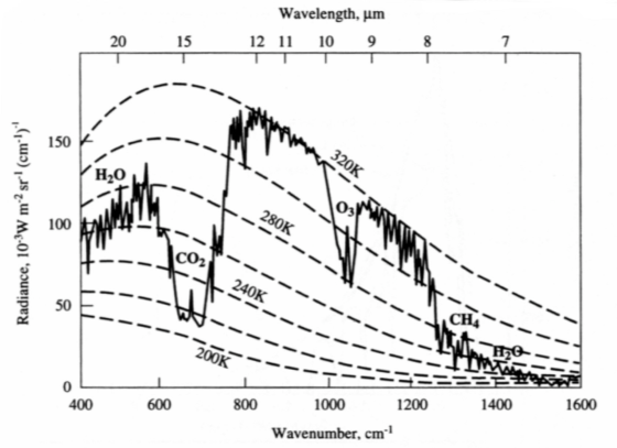
Figure 1: Radiation spectrum of the Earth as observed by a satellite over Africa.[3] Wavenumber is $1/\lambda$. Blackbody spectra at several temperatures are also shown. Multiply the numbers on the vertical axis by $\pi$ to obtain the radiation in $10^{-3}$W m${}^{-2}($cm${}^{-1})^{-1}$ (with m² now referring to the surface of the Earth instead of the satellite antenna).

3 A simple model

Let us begin with a simple model. From observations we know that, to high accuracy, there is an equilibrium between incident solar power and radiated infrared power. Therefore

$$\frac{1}{4}\epsilon_{v}I_{Sun}=\epsilon_{IR}\sigma T^{4},$$ (1)

where $I_{Sun}=1368$W/m² is the solar constant, $\epsilon_{v}$ is the fraction of incident sun light power that is absorbed by the Earth, i.e. it is the “emissivity in the visible”, $\epsilon_{IR}$ is the emissivity in the infrared, $\sigma=5.67\times 10^{-8}$Wm^-2K^-4 is the Stefan-Boltzmann constant, and $T$ is the temperature of the surface of the Earth in degrees Kelvin. The factor $\frac{1}{4}$ was explained in Section 2.

We note that if $\epsilon_{v}=\epsilon_{IR}$ the equilibrium temperature is 279K, quite close to the observed mean temperature of 288K.

From the data presented in Section 2 we conclude that $\epsilon_{v}\approx 0.69$ for the Earth as a whole, $\epsilon_{v}\approx 0.55$ for areas covered by clouds (it varies from 0.6 for cirrus to 0.1 for cumulonimbus), $\epsilon_{v}\approx 0.9$ for cloudless ground, and $\epsilon_{v}\approx 0.2$ for snow. Because snow is mostly at high latitude we sometimes replace $\epsilon_{v}\approx 0.1$ for snow.

From the data presented in Section 2 we estimate that $\epsilon_{IR}\approx 0.605$ for the Earth as a whole, $\epsilon_{IR}\approx 0.56$ for areas covered by clouds, $\epsilon_{IR}\approx 0.69$ for cloudless ground, and $\epsilon_{IR}\approx 0.3$ for snow.

These “effective” emissivities are valid for the model of this Section, i.e. an Earth surface characterized by a single temperature, and includes the atmosphere with its greenhouse gases. The model is too crude to account for all observations, so these effective emissivities are approximate. A summary of effective emissivities is presented in Table 1. In the last column of the table we show the equilibrium temperature for 100% coverage of black body, cloudless ground, clouds or snow. The last row shows the world average.

	infrared	visible	$T$ for 100% cover
black body	1.00	1.00	279K
cloudless ground	$\approx 0.69$	0.90	298K
clouds	$\approx 0.56$	0.55	278K
snow	$\approx 0.30$	0.10 (0.20)	212K (252K)
whole Earth	0.605	0.69	288K

Table 1: Effective emissivities for infrared and visible radiation. The last column shows the temperature corresponding to a 100% cover of black body, cloudless ground, cloud or snow. The last row corresponds to 50% cloud cover, 5% snow cover, leaving 45% clear ground. The measured average temperature is 288K.

4 Two box model

Figure 2 shows two boxes: one for the upper atmosphere at temperature $T_{2}$, and one for the surface and lower atmosphere at temperature $T$.[1] The surface radiates $\approx\sigma T^{4}$. A fraction $1-\epsilon$ of this radiation gets through the upper atmosphere (this is the infrared window), and a fraction $\epsilon$ is absorbed by greenhouse gases and aerosols in the atmosphere. The upper atmosphere radiates $\epsilon\sigma T_{2}^{4}$ back to the lower atmosphere, and $\epsilon\sigma T_{2}^{4}$ out to space. The total radiation out to space is

$$\sigma T^{4}-\epsilon\sigma\left(T^{4}-T_{2}^{4}\right).$$ (2)

The last term reduces the infrared emission of the Earth (at a given $T$) because the upper atmosphere is colder than the surface. This last term is the greenhouse effect. The effective emissivity is

$$\epsilon_{IR}=1-\epsilon\left[1-\left(\frac{T_{2}}{T}\right)^{4}\right].$$ (3)

We estimate $\epsilon\approx 0.813$ (see next section). For $T=288$K we obtain $T_{2}\approx 244$K. Note that heating of the upper atmosphere reduces the greenhouse effect. Adding greenhouse gases to the atmosphere has two opposing effects on $T$: $\epsilon$ increases and $T_{2}$ increases.

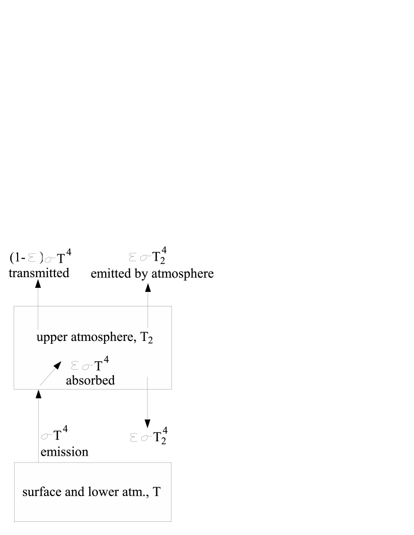
Figure 2: Two-box model of the greenhouse effect.[1]

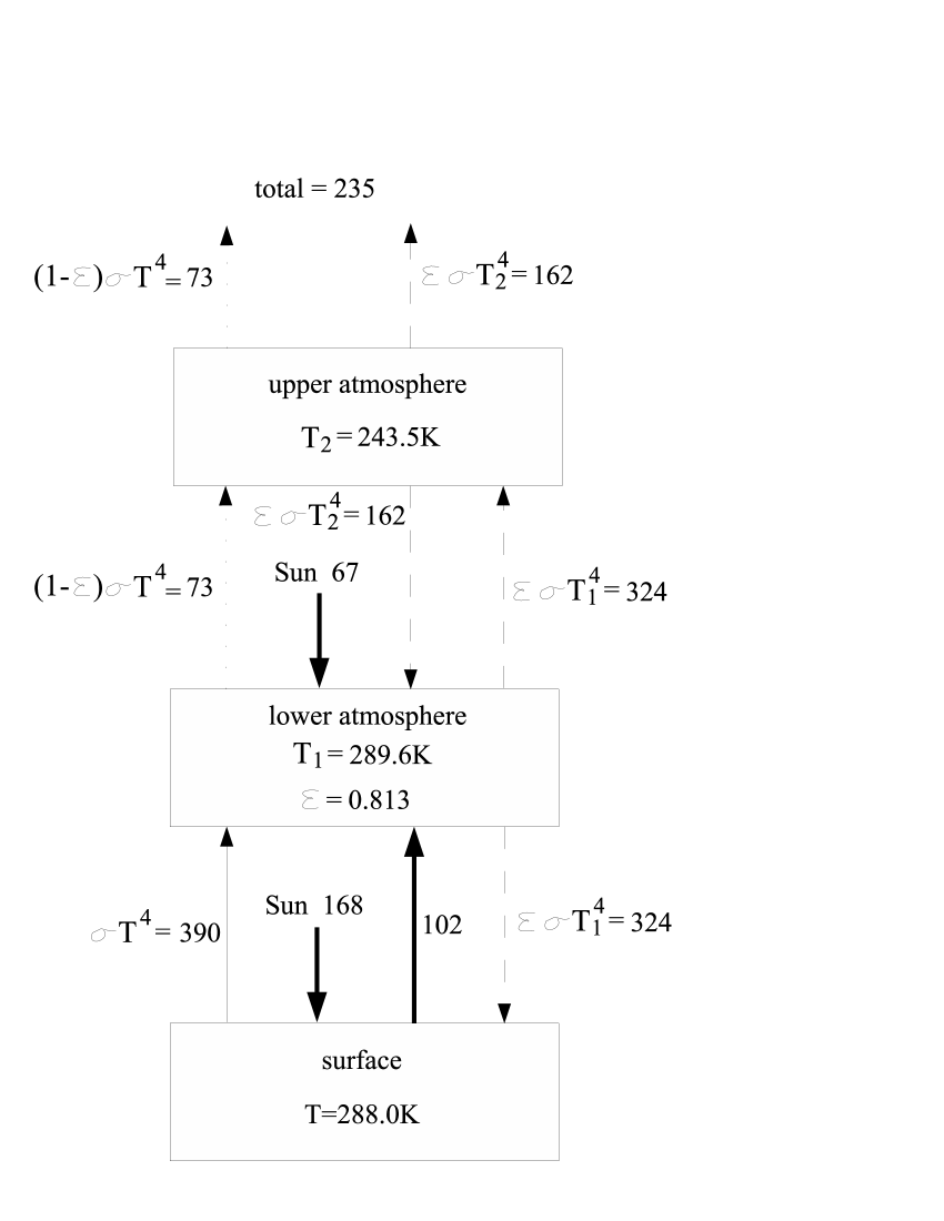
Figure 3: Three-box model of the greenhouse effect. The numbers are in units of W/m². Dotted lines correspond to the infrared window, while dashed lines correspond to frequencies absorbed or emitted by greenhouse gases in the atmosphere (mainly $H_{2}O$, $CO_{2}$ and ozone). Thermals, evaporation and transpiration are estimated to transport $102$W/m².

5 Three box model

The three box model is shown in Figure 3. The boxes are the surface of the Earth at temperature $T$, the lower atmosphere at temperature $T_{1}$, and the upper atmosphere at temperature $T_{2}$. The total radiation to space is equal to the total solar radiation absorbed ($235$W/m²), which we assume independent of the concentration of $CO_{2}$. The solar power absorbed per unit area is $168$W/m² by the surface, and $67$W/m² by the atmosphere. Thermals, evaporation and transpiration are estimated to transport $102$W/m².[1] The atmosphere absorbs radiation at frequencies near vibration resonances of the greenhouse gases, mainly $H_{2}O$, $CO_{2}$ and ozone. The fraction of infrared radiation absorbed is $\epsilon$. The atmosphere also radiates at these frequencies. The emissivity of the surface in the infrared is taken to be 1. The sum of powers entering each box is zero. The greenhouse effect is due to the low temperature of the upper atmosphere, so that emission to space is reduced at frequencies near resonances as shown in Figure 1.

$\epsilon$	$T$	$T_{1}$	$T_{2}$	comment
0.0	253.72K	n.a.	n.a.	235W/m2 radiation, no atmosphere
0.05	238.94K	452.5K	380.5K
0.3	250.51K	310.1K	260.8K
0.5	262.20K	290.5K	244.3K	model breaks down for $\epsilon<0.5$
0.6	269.20K	287.3K	241.6K
0.7	277.24K	286.9K	241.3K
0.8	286.65K	289.1K	243.1K
0.813	288.00K	289.6K	243.5K	290ppm $CO_{2}$
0.833	290.14K	290.4K	244.2K	580ppm $CO_{2}$
0.9	297.91K	293.9K	247.1K
1.0	311.81K	301.7K	253.7K	opaque atmosphere

Table 2: Temperatures of the surface ($T$), lower atmosphere ($T_{1}$), and upper atmosphere ($T_{2}$) in the three box model as a function of the emissivity of the atmosphere in the infrared ($\epsilon$). The absorbed Sun power and power of thermals, evaporation and transpiration are assumed to be constant (independent of the concentration of $CO_{2}$).

In Table 2 we show the temperatures as a function of the emissivity of the atmosphere in the infrared ($\epsilon$). The absorbed sun power and power of thermals, evaporation and transpiration are assumed to be constant (independent of the concentration of $CO_{2}$), so the model breaks down for $\epsilon\leq 0.5$ (with no atmosphere we should obtain $T=253.72$K for 235W/m² black-body radiation).

It has been estimated that doubling the concentration of $CO_{2}$ from (290ppm to 580ppm) decreases the radiation to space by $3.75\pm 0.25$W/m²[1] (before temperatures are allowed to adjust) which corresponds to increasing $\epsilon$ from 0.813 to 0.833. Note, in Table 2, that doubling the concentration of $CO_{2}$ raises the surface temperature $T$ by 2.1K. Do we trust this result? No! Most of the radiation to space is from the upper atmosphere. The temperature of the upper atmosphere may change with $CO_{2}$ concentration due to energy fluxes or absorptions not considered in this simple model. Also the solar inputs and power of thermals, evaporation and transpiration surely depend directly or indirectly on the $CO_{2}$ concentration (by changing $T$ and $T_{1}$).

6 Global warming from Earth emission spectra

Let us try a different approach that relies only on the Earth emission spectra shown in Figure 1. We estimate the increase in surface temperature due to a doubling of the concentration of $CO_{2}$ (from 290ppm to 580ppm). We take the average Earth temperature to be 288K (instead of the 320K of Africa shown in Figure 1).

$CO_{2}$ has two absorption bands in the tail of the solar spectrum, which absorb $\approx 0.8$W/m². We will neglect this absorption (a correction could be applied later). Increasing the concentration of $CO_{2}$ will widen the absorption resonance seen in Figure 1. How will the spectra respond? If the Earth albedo remains constant, then the area below the spectra in Figure 1 will remain constant. Then the spectra will respond by increasing (or in general, modifying) the surface temperature, and/or the water emission temperature ($T_{H_{2}O}\approx 260$K), and/or the $CO_{2}$ emission temperature ($T_{CO_{2}}\approx 215$K). Table 2 suggests that $T_{1}$ and $T_{2}$ vary less than the surface temperature $T$. So, in this section, without much justification, we will assume that (i) $T_{H_{2}O}$ and $T_{CO_{2}}$ remain constant, and (ii) the Earth albedo remains constant. So, in this approximation, the only response to the widening of the $CO_{2}$ absorption resonance is to increase the surface temperature to conserve the area under the spectrum in Figure 1.

Let us estimate the widening of the $CO_{2}$ resonance using only the data in Figure 1. This widening in W/m² (before any temperature has a time to react) is called “radiative forcing”. We label points of transmittance equal to 1, 0.7, 0.5, 0.25, 0.06, 0.004 and 0.0 along the side slopes of the absorption resonance, and then shift them downward (at constant wave number). The result is a radiative forcing $\approx 4$W/m². The corresponding change in surface temperature, in responce to a doubling of the concentration of $CO_{2}$, with the assumptions discussed above, is $\approx 2.5$K.

Another estimate would let $T$ and $T_{H_{2}O}$ vary by the same amount, while $T_{CO_{2}}$ remains constant. The corresponding warming is $\approx 1.3$K.

7 Detailed models

The results presented in this section were obtained from [1]. The surface and troposphere are tightly coupled (by non-radiative heat exchanges), while the coupling between the troposphere and stratosphere is relatively weak. For this reason changes in the surface temperature are largely determined by changes in the net (incoming minus outgoing) radiation at the tropopause (at an altitude between 10 and 20 km). This change in net radiation at the tropopause per unit surface area (before any temperatures are allowed to change), $\Delta R$, is called “radiative forcing”. The change in surface temperature is expressed as $\Delta T=\Delta R/\lambda$, where $\lambda$ is the “radiative damping”. If the Earth were a blackbody (radiating the same amount as the Earth), then $\lambda=3.7$Wm^-2K^-1. However due to various feedback effects, it is estimated, using detailed models, that $\lambda=2.0\pm 0.5$Wm^-2K^-1.[1] So the net feedbacks are positive.

The change in radiative forcing and surface temperature, due to changes in composition of the atmosphere since the pre-industrial period until 1995, is estimated by detailed models[1] to be $\Delta R=2.6\pm 0.6$Wm^-2 and $\Delta T=1.3\pm 0.44$K due to all greenhouse gases (about half of this is due to $P_{CO_{2}}$ increasing from 290ppm to 350ppm), and $\Delta R=-1.9\pm 1.1$Wm^-2 and $\Delta T=-1.0\pm 0.6$K due to all aerosols (we have added errors in quadrature). Deforestation changes the albedo of the Earth, causing a change of temperature $\approx-0.4$K.[4] So we do not know wether the increase of greenhouse gases, aerosols and deforestation has a net heating or cooling effect.

Let us now consider a doubling of the pre-industrial concentration of $CO_{2}$ (from 290ppm to 580ppm). The change in radiative forcing is $\Delta R=3.75\pm 0.25$Wm^-2[1] and the corresponding change of surface temperature is $\Delta T=1.9\pm 0.5$K. This result, obtained from detailed models[1] is in agreement with paleo-climate and historical data (and with our back-of-the-envelope estimates of Sections 5 and 6). In comparison, the change in temperature since the “little-ice-age” (1700) to the present (1995) has been $\approx 1.2$K.[5] It is worth mentioning that various detailed models obtain $\Delta T$ in the range from 1.3K to 4.8K for doubling of $CO_{2}$[1]. The range of results is large so this is a difficult problem that does not seem to converge: as the model becomes more complex, the uncertainties appear to increase!

8 Ice ages

For given emissivities, the Earth temperature is stable because an increase in temperature causes an increase in the infrared radiation, which in turn brings the temperature back to its equilibrium value. However, the equilibrium temperature depends on the emissivities. For example, a world-wide snow storm could result in a shift of the equilibrium temperature from 288K to as low as 252K, see Table 1, which would prevent snow from melting. In this way an ice age might begin.

The mean annual temperature averaged over the Earth fluctuates from year to year with a standard deviation of about $\approx 0.22^{0}$C (during the 20’th century). Inter-glacial periods last typically $\approx 50$ thousand years. With 50% probability we expect a fluctuation of at least 4.2 standard deviations in 50000 tries. This corresponds to $\approx 1^{0}$C. Is such a world-wide temperature fluctuation sufficient to throw us into an ice age?

To get out of an ice age, an event is needed to change the emissivities, perhaps volcanic eruptions (or meteorite impacts) that cover snow with ash. Table 3 is a list of the largest known volcanic eruptions in the last million years. Each one of them (except perhaps Taupo in isolated and tropical New Zealand) corresponds (within errors) to a transition from a glacial to an interglacial period, see Figure 4. It is interesting to note that an explosion that ejects $2\times 10^{15}$kg corresponds to an average of 4kg$\cdot$m^-2 over the entire Earth, so that such an event could have a sizable effect on the albedo. If the volcanic origin of the transitions is correct, we should find evidence for other large eruptions at approximately 770, 430, 340, 270 and 140 thousand years ago. Note however that volcanic explosions have a short-term cooling effect.[4]

On 4 November 2002 the volcano El Reventador in Ecuador exploded and covered Cayambe with ash. Two years later we see a barren Cayambe with large patches of glacier gone. Similarly, volcanic ash from Tungurahua has been falling on Chimborazo for the last few years. Chimborazo also looks barren compared with what it used to be.

Caldera name	ejected mass [$10^{15}$kg]	date [$10^{3}$ years ago]
Toba (Indonesia)	6.9	74
Yellowstone (Wyoming, USA)	2.2	600
Porsea (Toba, Indonesia)	2.0	790
Taupo (New Zealand)	1.3	26.5
Long Valley (California, USA)	1.2	700

Table 3: Large explosive volcanic eruptions in the last million years.[6]

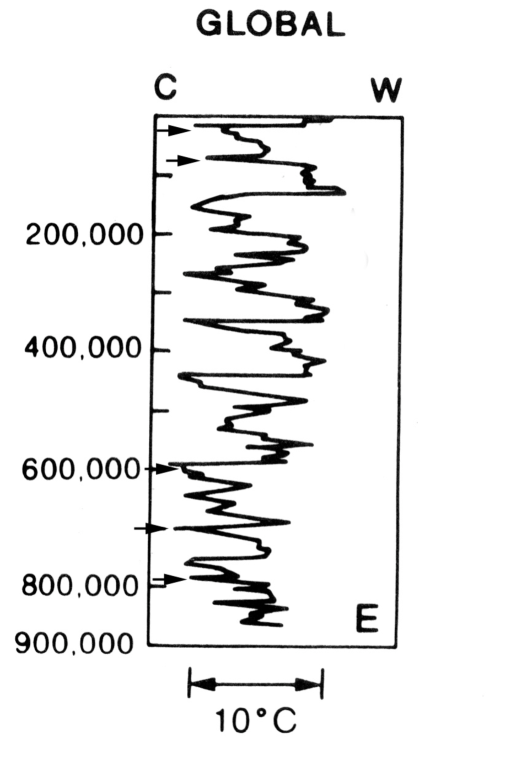
Figure 4: Ice-core temperature data of the last 900 thousand years[2], compared with the largest known volcanic explosions in that period (arrows)[6].

9 Width of the $15\mu$m line of $CO_{2}$.

The $CO_{2}$ molecule is linear, and has three normal modes of oscillation. They have wavelengths of $15\mu$m, 7.46$\mu$m and 4.26$\mu$m. The mode with wavelength 7.46$\mu$m has no dipole moment and does not couple to electromagnetic radiation. The mode with wavelength 4.26$\mu$m barely overlaps the black-body radiation spectrum of the Earth. So the important spectral line has a wavelength $\lambda=15\mu$m. We calculate the half-width of this line (neglecting molecule collisions) at the points of half power to be $\Delta\lambda/\lambda\approx 10^{-13}$.

Let us consider molecule collisions. The calculated mean free path at a pressure of one atmosphere is $l\approx 1\mu$m, the rms thermal velocity of $CO_{2}$ is $v=400$m/s at 300K, and the mean time between collisions is $\tau\approx 2.5$ns. If the time between collisions is $t$, then the half-width of the spectral line between points of half power is $\Delta\lambda/\lambda\approx 0.45\lambda/(ct)$. For $t=2.5$ns the result is $\Delta\lambda/\lambda\approx 10^{-5}$. The probability that $t$ is in the interval $dt$ is $\tau^{-1}\exp[-t/\tau]\cdot dt$. So the spectral line has very long tails that absorb electromagnetic radiation. These long tails explain the wide absorption band of $CO_{2}$ seen by satellites.

We have calculated the half-width $\Delta\lambda$ of the window corresponding to the $\lambda=15\mu$m line of $CO_{2}$ at which the power per unit area getting through the atmosphere drops by a factor $e^{-2}$:

$$\Delta\lambda\approx\frac{\lambda^{2}q}{4\pi c}\left[\frac{2P_{CO_{2}}L\eta_{0}}{kTm\tau}\right]^{\frac{1}{2}},$$ (4)

where $\eta_{0}=120\pi$ Ohm is the impedance of free space, $P_{CO_{2}}$ is the partial pressure of $CO_{2}$ at sea level, $L=kT/(Mg)=5550$m is the altitude at which the partial pressure of $CO_{2}$ drops by a factor $e^{-1}$, $c$ is the velocity of light, $m$ is the reduced mass of a carbon atom oscillating against two oxygen atoms, $T$ is the absolute temperature, $\tau$ is the mean time between collisions of $CO_{2}$ molecules, and $q$ is the effective charge of the carbon in $CO_{2}$. Substituting numerical values we obtain $\Delta\lambda\approx 0.6\mu$m for 300ppm $CO_{2}$, in reasonable agreement with $\approx 1.0\mu$m measured by satellites. So we understand the long tails of the spectral line of $CO_{2}$. Note that doubling $P_{CO_{2}}$ increases $\Delta\lambda$ by a factor $\sqrt{2}$.

pH	$CO_{2}$	$CO_{2}$	$HCO_{3}^{-}$	$HCO_{3}^{-}$	Gt of C	Gt of C
	$0^{0}$C	$25^{0}$C	$0^{0}$C	$25^{0}$C	$0^{0}$C	$25^{0}$C
7.0	$2.49\cdot 10^{-4}$	$1.04\cdot 10^{-4}$	$2.12\cdot 10^{-3}$	$1.43\cdot 10^{-3}$	843	550
7.4	$2.49\cdot 10^{-4}$	$1.04\cdot 10^{-4}$	$5.32\cdot 10^{-3}$	$3.60\cdot 10^{-3}$	1994	1325
8.3	$2.49\cdot 10^{-4}$	$1.04\cdot 10^{-4}$	$4.23\cdot 10^{-2}$	$2.86\cdot 10^{-2}$	15224	10270

Table 4: The columns contain the ocean pH; the number of kilograms of carbon per cubic meter of ocean at $0^{0}$C and $25^{0}$C in the form $CO_{2}$ and $HCO_{3}^{-}$[7]; and the corresponding total carbon in the upper 1000m of the oceans. The calculations correspond to 300ppm of $CO_{2}$ in the atmosphere. In comparison, the atmosphere with 300ppm of $CO_{2}$ contains 430Gt of carbon. Oceans have a pH between 7.4 and 8.3.[7]

10 Equilibrium of $CO_{2}$ between atmosphere and oceans

The chemistry of carbon in the oceans is beautifully described in [7]. We are interested in these two equations of chemical equilibrium:

$$[CO_{2}]=K_{H}P_{CO_{2}},$$ (5)

which describes the solution of $CO_{2}$ in sea water, and

$$[H^{+}][HCO_{3}^{-}]=K_{a1}[CO_{2}]$$ (6)

that describes the ionization of hydrated carbon dioxide. $P_{CO_{2}}$ is the partial pressure of $CO_{2}$ in the atmosphere (in atmospheres), and $[...]$ are concentrations in sea water (in mol per liter). The equilibrium constants have these values at $0^{0}$C ($25^{0}$C): $-\log K_{H}=1.16$ ($1.54$), and $-\log K_{a1}=6.07$ ($5.86$) for 0.7 ionic strength.[7] The calculations shown in Table 4 assume $P_{CO_{2}}=0.0003$atm (i.e.300ppm).

Assuming that the total carbon in the air and the top 1000m of the oceans is constant, and that 300ppm corresponds to $10^{0}$C and pH = 7.4 (8.3), we obtain that a $10^{0}$C increase in the sea water temperature produces an increase of $CO_{2}$ in the atmosphere of 40ppm (48ppm). In comparison, from Antarctic and Greenland ice cores, it is found that $9.5^{0}$C changes in temperature have been accompanied by $\approx 75$ppm change in $P_{CO_{2}}$.

In conclusion, we qualitatively understand the coupling of the pre-historic temperature with the atmospheric concentration of $CO_{2}$: an increase of ocean temperature reduces its solubility to $CO_{2}$, causing an increase of the atmospheric concentration of $CO_{2}$. The converse is not true: an increase of $75$ppm $CO_{2}$ would increase the temperature, due to the greenhouse effect, by only $\approx 0.8^{0}$C.

Let us now estimate the effect of acid rain due to a large volcanic explosion. Assume that $2\times 10^{15}$kg are ejected. Assume that 0.1% of this is sulfur (in any chemical form) that ends up as sulphuric acid in the oceans. The concentration of $H_{2}SO_{4}$ in the top 1000m of the oceans would be $1.8\cdot 10^{-4}$mmol/liter. We measured the pH of ocean water off the coast of Ecuador as a function of $H_{2}SO_{4}$ concentration: 7.3, 7.0, 6.3, and 5.5 for 0, 0.0084, 0.0211 and 0.0422mmol/liter respectively. So the change of pH is negligible ($\approx 0.006$), and the corresponding release of $CO_{2}$ by the oceans is also negligible.

11 A comment on the carbon cycle

It is observed that the concentration of $CO_{2}$ has increased linearly from 325ppm in 1970 to 375ppm in 2004.[8] If this increase continues at constant rate it will take about $\approx 140$ years to reach twice the pre-industrial concentration of 290ppm.

It is observed that the buildup of atmospheric $P_{CO_{2}}$ accurately follows the human emissions of $CO_{2}$ (due to burning of fossil fuels and the clearing of land for agricultural and urban use).[1] The factor of proportionality is observed to be 65%. The remaining 35% of emitted carbon apparently ends up in the surface (mixed) layer of the oceans and in bio-mass. No saturation is observed so far, so the time constant with which carbon reaches the deep oceans is in excess of 50 years (it is estimated that there are several time constants, some as long as 2000 years).[1]

There are enough world reserves of fossil fuels (gas, oil and coal) to last $\approx 150$ years at the present rate of consumption (6.5Gt C per year). Burning these reserves would increase $CO_{2}$ to three times the pre-industrial concentration assuming 65% of the emitted $CO_{2}$ ends up in the atmosphere. However, on these longer time scales it is estimated that 30% (instead of 65%) of the emitted $CO_{2}$ will remain in the atmosphere.[1] Thus we estimate that burning all of the remaining reserves of fossil fuels in the next 150 years or so, will result in twice the pre-industrial $CO_{2}$ concentration.

12 Time constant to reach $CO_{2}$ equilibrium with the oceans.

The solubility of $CO_{2}$ in the oceans decreases with increasing temperature. Consider a drop in the temperature of the oceans. With what time constant does the atmospheric concentration of $CO_{2}$ drop due to the increased absorption by the oceans? Here we assume that every $CO_{2}$ molecule colliding with the ocean surface “sticks” to the surface. The number of $CO_{2}$ molecules colliding with a square meter of ocean surface per second is[9]

$$R=\sqrt{\frac{kT}{2\pi M}}\frac{P_{CO_{2}}}{kT}=7\cdot 10^{23}\textrm{m}^{-2}\textrm{s}^{-1}.$$ (7)

The number of $CO_{2}$ molecules in the atmosphere per square meter is $P_{CO_{2}}/(Mg)=4\cdot 10^{25}$m^-2. So the time constant for absorption of $CO_{2}$ by very cold oceans is $\approx 90$s (we have taken account that 0.7 of the surface of the Earth is covered by oceans). So equilibrium of $CO_{2}$ and the oceans is very short if we neglect diffusion of $CO_{2}$ through the atmosphere.

Let us now consider diffusion. The partial pressure of $CO_{2}$ decreases with altitude exponentially with a characteristic height $L=kT/(Mg)=5550$m. How long does it take a molecule of $CO_{2}$ to diffuse 5550m through the atmosphere? The result is $t=L^{2}/(vl)\approx 2400$ years. This result assumes no convection. Convection will reduce this time considerably. In fact, the flux of carbon from the atmosphere to the oceans and vice versa is enough to replace all the atmospheric carbon in 6 years.[1] So, on time scales of interest, the partial pressure of $CO_{2}$ in the atmosphere is proportional to the concentration of $CO_{2}$ in the surface water of the oceans: they are in equilibrium.

13 The carbon cycle in the Amazon rain forest

In the process of photosynthesis, a plant takes $CO_{2}$ from the air, breaks it up using solar energy, and releases $O_{2}$ back to the atmosphere. The carbon attaches to water to form carbohydrates $(CH_{2}O)_{n}$, which is what plants are made of. So, for every molecule of oxygen released to the atmosphere, there remains one atom of carbon in the plant. What happens to the carbon when the plant dies? There are three alternatives: the carbon can (i) return to the atmosphere, (ii) accumulate on the ground, or (iii) end up in the oceans.

The photosynthesis process can occur in both directions. Examples of photosynthesis in reverse direction are combustion when we burn wood, respiration, and decomposition by aerobic bacteria. In these processes the carbon of the plant becomes attached to oxygen from the air, and is returned to the atmosphere as $CO_{2}$. Note that no net oxygen is produced: the oxygen released to the atmosphere during the plant growth is consumed during the plant aerobic decay.

The carbon can end up in the soil, either as partially decomposed organic matter (humus), as hydrocarbons or as coal. If the plant dies in a medium that lacks oxygen, such as in oceans, lakes, rivers, swamps or under volcanic ash, the anaerobic bacteria have a chance to decompose the plant (without the competition from aerobic bacteria). The anaerobic bacteria produce methane (“swamp gas”), carbonic acids, bicarbonates, and humic acids. The methane can escape to the atmosphere, or under enough pressure and temperature, can polymerize into hydrocarbons or can be crushed into coal.

The carbon can be washed down the rivers, in the form of carbonic acids, bicarbonates, and humic acids which are soluble in water. The rivers in the Amazon basin are dark due to the humic acids.

The Amazon rain forest has humus only in the first few centimeters of soil. So we neglect alternative (ii). To quantify alternative (iii), we took samples of water of several tributaries of the Amazon river (Napo Alto, Napo Bajo, San Francisco and Tiputini) and measured the concentration of bicarbonate (0.71 mol/m³) and carbonic acid (0.11 mol/m³). Assuming that these concentrations are typical of the Amazon river, and multiplying by the yearly discharge of the river, we obtain the carbon discharged to the Atlantic ocean by the Amazon river: 50 million (metric) tonnes per year. In total, the Amazon basin fixes about 10 billion brute tonnes of carbon per year. So, about 99.5% of this carbon returns to the atmosphere due to the aerobic decomposition of organic matter, while only about 0.5% is washed down the rivers into the Atlantic ocean.

It is interesting to compare these numbers with the world energy-related release of carbon dioxide from the consumption of oil, gas and coal: 24 billion tonnes in 2004. This corresponds to 6.5 billion tonnes of carbon per year. So the Amazon basin can transfer, from the atmosphere to the oceans, one year’s worth of carbon dioxide emission in 130 years!

14 Conclusions

With some degree of confidence, we arrive at the following conclusions.

1. Ever since we have accurate measurements of the temperature of the atmosphere, i.e. since 1702, we observe a global increase of temperature of about 0.4⁰C per century. This warming does not accelerate in the second half of the XX century. In fact, we see no statistically significant global warming since 1940.[2, 5] We observe no correlation of the global temperature with the consumption of oil, coal and gas, or with population. The atmospheric concentrations of $CO_{2}$ begins to increase around 1940[2] when oil consumption takes off, yet we observe no corresponding increase of the slope of global warming.[2, 5, 10] Some studies suggest that this is due to a balance between the heating effect of $CO_{2}$ and the cooling effects of aerosols and deforestation.[1, 4] From the data it is concluded that the accumulated effect of humankind on the global temperature until 1990 is not statistically significant: $0.0\pm 0.1^{0}$C.[5] So, the observed global warming since 1702 is part of the natural variability of the climate as we pull out of the “little ice age” three centuries ago.

2. The pre-industrial concentration of $CO_{2}$ in the atmosphere was $\approx 290$ ppm in 1800. It has since increased to 375 ppm in 2004.[8] There is convincing evidence that this increase is due to burning of fossil fuels (and forrests, and the manufacture of cement).

3. Detailed models estimate that the changes of atmospheric composition since pre-industrial times up to 1995 produce a change of temperature of $1.3\pm 0.44$K due to all greenhouse gases (about half of this is from $CO_{2}$), $-1.0\pm 0.6$K due to aerosols[1], and $\approx-0.4$K due to the change of albedo caused by deforestation[4]. So we do not know if human activity heats or cools the Earth. As indicated above, no significant net change has been observed.

4. The increase of the concentration of $CO_{2}$ in the atmosphere accurately tracks the burning of fossil fuels (and forrests). Two thirds of the carbon burned ends up in the atmosphere as $CO_{2}$, and the remaining third ends up dissolved in the surface layer of the oceans (the time constant for this dissolution is about 6 years). The fraction of excess carbon in the atmosphere should decrease to one third in about 50 years as more carbon is incorporated into the oceans (as $CO_{2}$, $HCO_{3}^{-}$, $CO_{3}^{--}$, $CaCO_{3}$), and in the land and marine biota. The last third of the excess $CO_{2}$ in the atmosphere is expected to return to the deep oceans and become buried as elemental carbon and as carbonates with several time constants ranging from hundreds to thousands of years.[1]

5. Burning all of the remaining economically viable reserves of oil, gas and coal over the next 150 years or so will approximately double the pre-industrial atmospheric concentration of $CO_{2}$. The global warming due to a doubling of the concentration of $CO_{2}$ is expected to increase the average surface air temperature by 1.3K to 4.8K.[1] The increase of temperature is expected to be higher than average at higher latitudes (and lower than average at low latitudes). The heating effect of $CO_{2}$ is obvious when we look at the Earth emission spectra shown in Figure 1. The range of results is large, so global warming is a difficult problem that does not seem to converge: as the models become more complex, the uncertainties appear to increase!

6. Ice core samples indicate that $CO_{2}$ concentration and temperature are well correlated: a change of temperature by 9.5⁰C corresponds to a change in $CO_{2}$ concentration from 195ppm to 270ppm.[2] Does the change of $CO_{2}$ concentration cause the change of temperature (by the greenhouse effect), or does the change of temperature cause the change of $CO_{2}$ concentration (due to the temperature dependence of the solubility of carbon in the oceans)? Due to the greenhouse effect, an increase of $CO_{2}$ concentration from 195ppm to 270ppm would cause an increase in temperature of $\approx 0.8^{0}$C, much too small to account for the observed change in temperature. Conversely, an increase of $9.5^{0}$C of the temperature of the upper 1000m of the oceans would increase the atmospheric concentration of $CO_{2}$ by $\approx 44$ppm (depending on the ocean pH). So it is plausible that the changes of temperature of the oceans caused the pre-historic changes of atmospheric $CO_{2}$ concentration.

7. Data suggests that large volcanic explosions can trigger transitions from glacial to interglacial climates, by covering ice with volcanic ash, thereby changing the equilibrium temperature of the Earth as seen in Table 1.

8. Photosynthesis in the Amazon basin fixes $\approx 10$ billion tonnes of carbon per year. However, aerobic decay releases almost all of this carbon back to the atmosphere as $CO_{2}$. The balance, $\approx 50$ million tonnes of carbon per year, is discharged to the Atlantic Ocean in the form of carbonic acids, bicarbonates, and humic acids.

References

- [1] L.D. Danny Harvey, “Global warming. The hard science”, Pearson Education Limited (2000)
- [2] Roger G. Barry and Richard J. Chorley, “Atmosphere, weather and climate”, sixth edition, Routledge (1992)
- [3] Hanel et. al., Geophys.Res. 77:2629-2641 (1972)
- [4] Eva Bauer, Martin Claussen, and Victor Brovkin, “Assessing climate forcings of the Earth system for the past millennium”, Geophysical Research Letters, 30, No. 6, 1276 (2003)
- [5] E. X. Albán, B. Hoeneisen, “Global warming: What does the data tell us?”, arxiv, physics/0210095 (2002)
- [6] “List of the largest explosive eruptions on Earth”, from http://www-volcano.geog.cam.ac.uk/database/list.html.
- [7] James N. Butler, “Carbon dioxide equilibria and their applications”, Addison-Wesley Publishing Company (1982)
- [8] Mauna Loa Observatory data.
- [9] Bruce Hoeneisen, “Thermal Physics”, EMText (1993)
- [10] Arthur B. Robinson, Sallie L. Baliunas, Willie Soon, Zachary W. Robinson, “Environmental effects of increased atmospheric carbon dioxide”.