Realizing a stable magnetic double-well potential on an atom chip

Abstract

We discuss design considerations and the realization of a magnetic double-well potential on an atom chip using current-carrying wires. Stability requirements for the trapping potential lead to a typical size of order microns for such a device. We also present experiments using the device to manipulate cold, trapped atoms.

1 Introduction

Progress in the fabrication and use of atom chips has been rapid in the past few years Folmanrevue . Two notable recent results concern the coherent manipulation of atomic ensembles on the chip: Ref. treutlein:2004 reported the coherent superposition of different internal degrees of freedom while in wang:2004 ; zimmermann:private a coherent beam splitter and interferometer using Bragg scattering was reported. In the same vein, the observation of a coherent ensemble in a chip-based double-well potential also represents a significant milestone. The dynamics of a Bose-Einstein condensate in a double-well potential has attracted an enormous amount of theoretical attention theory , in part because one can thus realize the analog of a Josephson junction. Indeed, coherent oscillations of atoms in a laser induced double-well potential have recently been observed albiez:2005 . In addition, the observation of an oscillation in a double-well amounts to the realization of a coherent beam splitter which promises to be enormously useful in future atom interferometers based on atom chips cassetari:2000 ; hinds:2001 ; hansel:2001c ; andersson:2002 .

In this paper, we discuss progress towards the realization of coherent oscillations on an atom chip. We begin with some theoretical considerations concerning atoms in double-well potentials and show that a configuration with two elongated Bose-Einstein condensates that are coupled along their entire length allows one to achieve a variety of oscillation regimes. Then, we will discuss design considerations which take into account stability requirements for the trapping potentials in the transverse direction. Fluctuations in the external magnetic fields impose a typical size less than or on the order of microns on the double-well. Atom chips implemented with current-carrying wires are well suited to elongated geometry and the micron size scale. After these general considerations, we discuss a particular realization of a magnetic double-well potential which has been constructed in our laboratory. Our device has much in common with the proposal of Ref. hinds:2001 , but we believe it represents an improvement over the first proposal in that it is quite robust against technical noise in the various currents. We will also show some initial observations with the device using trapped ⁸⁷Rb atoms.

2 Dynamics of two elongated Bose-Einstein condensates coupled by tunneling

The dynamics of a Bose-Einstein condensate in a double-well potential has been widely discussed in the literature theory . In this section, we will review some of the basic results and apply them to the case of two elongated condensates coupled by tunneling along their entire length $L$.

We assume the trapping potential can be written as the sum of a weakly confining longitudinal potential $V_{l}(z)$ and a two dimensional (2D) double-well in the transverse direction $V_{r}(\mathbf{r})$. We characterize the two transverse potential wells by the harmonic oscillator frequency at their centers, $\omega_{0}$. We also assume that the longitudinal motion of the atoms is decoupled from the transverse motion, so that we may restrict ourselves to a 2D problem. As discussed in bouchoule:2005 , this assumption is not always valid, but it gives a useful insight into the relevant parameters of the problem and how they affect the design of the experiment.

Considering the motion of a single atom, the lowest two energy states of the 2D potential $V_{r}$ are symmetric and antisymmetric states, $|\phi_{s}\rangle$ and $|\phi_{a}\rangle$. The energy splitting $\hbar\,\delta$ between them is related to the tunneling matrix element between the states describing a particle in the right and left wells, $|\phi_{r}\rangle$ and $|\phi_{l}\rangle$. When including atom-atom interactions, we assume that the longitudinal linear density $n_{1}$ is low enough to satisfy $n_{1}\,a\ll 1$ where $a$ is the $s$-wave scattering length. In this case, the interaction energy is small compared to the characteristic energy $\hbar\,\omega_{0}$ of the transverse motion, and in a mean field approximation the eigenstates of the Gross-Pitaevskii equation are identical to the single particle eigenstates. The tunneling rate $\delta$ is unchanged in this approximation. If in addition, $\delta\ll\omega_{0}$, the two mode approximation in which one considers only the states $|\phi_{s}\rangle$ and $|\phi_{a}\rangle$ (or $|\phi_{l}\rangle$ and $|\phi_{r}\rangle$) is valid.

We now define two characteristic energies $E_{J}$ and $E_{C}$. The Josephson energy $E_{J}=N\,\hbar\,\delta/2$ characterizes the strength of the tunneling between the wells. The charging energy $E_{C}=4\,\hbar\,\omega_{0}\,a/L$ is analogous to the charging energy in a superconducting Josephson junction and characterizes the strength of the inter atomic interaction in each well. The properties of the system depend drastically on the ratio $E_{C}/E_{J}$ theory . For the considered elongated geometry, this ratio is equal to $(4\,n_{1}\,a)\times(\omega_{0}/\delta)\times 1/N^{2}$. A ratio $\omega_{0}/\delta$ of 10 is enough to insure the validity of the two mode approximation. We have also assumed $n_{1}\,a\ll 1$ and since $N\gg 1$ we indeed obtain $E_{C}/E_{J}\ll 1$. This means that the phase difference between the two wells is well defined and that a mean field description of the system is valid.

In the mean field approximation, the transverse part of the atomic wavefunction can be written $|\phi\rangle=c_{l}\,|\phi_{l}\rangle+c_{r}\,|\phi_{r}\rangle$ where $c_{l}$ and $c_{r}$ are complex numbers. The atom number difference $\Delta N=(|c_{l}|^{2}-|c_{r}|^{2})/2$ and the phase difference $\Delta\theta=\arg(c_{l}/c_{r})$ evolve as the classically conjugate variables of a non rigid pendulum Hamiltonian smerzi:1997 . The solutions of the motion for $\Delta N$ and $\Delta\theta$ have been analytically solved smerzi:1997 ; raghavan:1999 . Depending on the ratio $E_{J}/(N^{2}\,E_{C})$, we distinguish two regimes: the Rabi regime ($E_{J}\gg N^{2}\,E_{C}$) and the Josephson regime ($E_{J}\ll N^{2}\,E_{C}$). For a fixed geometry ($L$, $\delta$ and $\omega_{0}$ fixed), the Rabi regime is delimited by $N\ll N_{C}$ where $N_{C}=\delta\,L/(4\,\omega_{0}\,a)$ while the Josephson regime corresponds to $N\gg N_{C}$. For a box like potential of length $L=1$ mm and a ratio $\omega_{0}/\delta=10$, this number corresponds to $N_{C}=5000$ for ⁸⁷Rb atoms.

In the Rabi regime, an initial phase difference of $\pi/2$ leads to the maximal relative atom number difference $\Delta N/N=1/2$. In the Josephson regime, the signal $\Delta N/N$ is limited to $\sqrt{N_{C}/N}$. One motivation to attain the Rabi regime is to maximize the relative population difference. If tunneling is to be used as a beam splitting device in an atom interferometer, the Rabi regime is clearly favorable as it maximizes the measured signal. It is also important to note that the neglect of any longitudinal variations in the atom number difference or the relative phase is only valid deep in the Rabi regime bouchoule:2005 .

The specific geometry of two elongated Bose-Einstein condensates coupled by tunneling is of special interest since it allows one to tune the strength of the interaction compared to the tunneling energy by adjusting the longitudinal atomic density. This allows realization of experiments in both the Rabi regime and the Josephson regime. On the other hand a complication of the elongated geometry is the coupling between the transverse and longitudinal motions introduced by interactions between atoms. This coupling is responsible for dynamical longitudinal instabilities in presence of uniform Josephson oscillationsbouchoule:2005 . However, Ref. bouchoule:2005 predicts that a few Josephson oscillations periods should be visible before instabilities become too strong. Furthermore, the study of these instabilities may prove quite interesting in their own right. Other manifestations of the coupling between the transverse and the longitudinal motion may be observed. In particular, Josephson vortices are expected for large linear densityKaurov:2005 . These nonlinear phenomena are analogous to observations on long Josephson junctions in superconductors likharev:book .

3 Realization of a magnetic double-well potential

We now turn to some practical consideration concerning the realization of the transverse double-well potential $V_{r}(x,y)$ using a magnetic field. As first pointed out in hinds:2001 , a hexapolar magnetic field is a good starting point to produce such a potential. The hexapolar field can be written

$$\left\{\begin{array}[]{cccccc}B_{x}&=&A\,(y^{2}-x^{2})&=&-A\,r^{2}\,\cos 2\theta\\ B_{y}&=&2\,A\,x\,y&=&A\,r^{2}\,\sin 2\theta\,.\\ \end{array}\right.$$ (1)

where $A$ is a constant characterizing the strength of the hexapole. In the following, we write this constant $A=\alpha\,\mu_{0}\,I/(4\,\pi\,d^{3})$ where $I$ is the current used to create the hexapole, $d$ is the typical size of the current distribution creating the magnetic field (see Fig. 4) and $\alpha$ is a geometrical factor close to unity. Adding a uniform transverse magnetic field $\mathbf{b}=b(\cos\theta_{b}\,\mathbf{x}+\sin\theta_{b}\,\mathbf{y})$ will split the hexapole into two quadrupoles, thus realizing a double-well potential. The two minima are separated by a distance $2\,X_{0}$ where $X_{0}=\sqrt{b/A}$ and are located on a line making an angle $\theta_{b}/2$ with the $\mathbf{x}$-axis (see Fig. 1). Tilting the axis of the double-well allows one to null the gravitational energy shift which arises between the two wells if they are not at the same height. This shift has to be precisely cancelled to allow the observation of unperturbed phase oscillations in the double-well. For example, if the two wells are separated by a vertical distance of 1 $\mu$m the gravitational energy shift between the two wells leads to a phase difference of 13 rad.ms^-1 for ⁸⁷Rb.

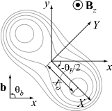
Figure 1: Adding a small magnetic field $\mathbf{b}$ to the magnetic hexapole described in Eq. 1 will split the hexapole into two quadrupoles. The distance between the two minima increases with $b$ and the direction along which the minima are split depends on the orientation of $\mathbf{b}$ as shown in the figure. We also have plotted lines of constant modulus of the total magnetic field (equipotential lines for the atoms).

In the rotated basis $(O,X,Y)$ (see Fig. 1), the modulus of the total magnetic field is

$$\mathbf{B}^{2}=2\,A\,b\,Y^{2}+2\,A\,X^{2}\,Y^{2}+A^{2}(X^{2}-X_{0}^{2})^{2}\,.$$ (2)

To prevent Majorana losses around each minimum, a uniform longitudinal magnetic field $B_{z}$ is added. Under the assumption $B_{z}\gg b$, the potential seen by an atom with a magnetic moment $\mu$ and a mass $m$ is

$$V(X,Y)\simeq\frac{m\,\omega_{0}^{2}}{4}Y^{2}+\frac{m\,\omega_{0}^{2}}{4\,X_{0}^{2}}X^{2}\,Y^{2}+\frac{m\,\omega_{0}^{2}}{8\,X_{0}^{2}}(X^{2}-X_{0}^{2})^{2}$$ (3)

with $\omega_{0}=\sqrt{4\,\mu\,A\,b/(m\,B_{z})}$.

Around each minimum $(X=\pm X_{0},Y=0)$, the potential is locally harmonic with a frequency $\omega_{0}$ and we denote $a_{0}=\sqrt{\hbar/(m\,\omega_{0})}$ the size of the ground state of this harmonic oscillator. On the $X$-axis, we recover the 1D double-well potential usually assumed in the literature. As seen in equation (3), the potential is entirely determined by the values of $\omega_{0}$ and $X_{0}$. We have computed the energy differences between the ground state and the two first excited states for a single atom as a function of these two parameters (see Fig. 2). The Bohr frequency $\omega_{1,0}$ is equal to the tunneling rate $\delta$. We calculate that a ratio $X_{0}/a_{0}=2.65$ ensures that $\omega_{2,0}=10\,\delta$, so that the two mode approximation is valid. Further calculations are made for a double-well potential fulfilling the condition $X_{0}/a_{0}=2.65$.

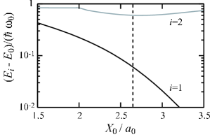
Figure 2: Bohr frequency between the ground state and the first two excited states of the double-well potential versus the spacing between the wells. The dashed line corresponds to $X_{0}=2.65\,a_{0}$ for which the Bohr frequency $\omega_{2,0}$ is ten times bigger than the tunneling rate $\delta=\omega_{1,0}$.

3.1 Stability of the double-well

We now turn to the analysis of the stability of the system with respect to fluctuations of magnetic field. We will impose two physical constraints: first we require a stability of 10% on the tunneling rate $\delta$ and second we impose a gravitational energy shift between the two wells of less than 10% of the tunneling energy. Assuming a perfectly stable hexapole and that fluctuations in the external fields can be kept below 1 mG, we will obtain constraints on the possible size of the current distribution $d$ and on the spacing between the two wells $X_{0}$.

The geometry of the magnetic double-well is determined by four experimental parameters: $I$ the current creating the hexapole, $d$ the size of the current distribution, $B_{z}$ the longitudinal magnetic field and $b$ the transverse field. To minimize the sensitivity of the system to magnetic field fluctuations, the current $I$ creating the hexapole should be maximized. If we suppose the wires that create the hexapole are part of an atom chip, the maximal current allowed in such wires before damage scales as $I=I_{0}(d/d_{0})^{3/2}$ groth:2004 . Henceforth we suppose that the current $I$ follows this scaling law and is not a free parameter anymore. Furthermore, the condition of the last section $X_{0}/a_{0}=2.65$ relates $b$ and $B_{z}$. Thus we are left with only two free parameters which may be chosen as the size of the source $d$ and the distance between the wells $X_{0}$. The experimental parameters $b$ and $B_{z}$ can be deduced afterwards.

We first calculate the variation $\Delta\delta$ of the tunneling rate due to longitudinal and transverse magnetic field fluctuations (respectively noted $\Delta B_{z}$ and $\Delta b$). From the numerical calculation of the tunneling rate shown in figure 2 we obtain

$$\frac{\Delta\delta}{\delta} = -2.40\,\frac{\Delta X_{0}}{X_{0}}-2.18\,\frac{\Delta\omega_{0}}{\omega_{0}}$$ (4)

$$= -4.27\,\frac{\Delta b}{b}+1.09\,\frac{\Delta B_{z}}{B_{z}}\,.$$ (5)

If we require a relative stability of 10% on the tunneling rate, the required relative stability for the magnetic fields $b$ and $B_{z}$ is approximately the same and is easily achievable with a standard experimental setup. However fluctuations due to the electromagnetic environment may be problematic. Within the assumption $B_{z}\gg b$, only the first term in equation (5) contributes. Thus we have

$$\frac{\Delta\delta}{\delta}\simeq-4.27\,\frac{4\,\pi d^{3}}{\alpha\,\mu_{0}\,I\,X_{0}^{2}}\Delta b\,.$$ (6)

Using the scaling law stated above for the current creating the hexapole, we finally obtain the following expression for the tunneling rate fluctuations due to variations of the transverse magnetic field

$$\frac{\Delta\delta}{\delta}\simeq-4.27\,\left(\frac{4\,\pi\,d_{0}^{3/2}}{\alpha\,\mu_{0}\,I_{0}}\right)\frac{d^{3/2}}{X_{0}^{2}}\,\Delta b\,.$$ (7)

We require a relative stability of 10% for the tunneling rate given an amplitude $\Delta b=1$ mG for the magnetic field fluctuations. This limits the possible values for $X_{0}$ and $d$ to the domain above the continuous line plotted in figure 3. For the numerical calculation, we have used a geometrical factor $\alpha=4/\sqrt{3}$ (see Sect. 4) and the following values for $I_{0}$ and $d_{0}$. A maximal current of $I_{0}=20$ mA is reasonable for gold wires having a square section of 500 nm$\,\times\,$500 nm which are deposited on an oxidized silicon wafer groth:2004 . Such wires can be used in a configuration where the typical distance between wires is $d_{0}=5$ $\mu$m.

We now turn to the calculation of the fluctuations of the gravitational energy shift between the two wells. Transverse magnetic field fluctuations lead to fluctuations $\Delta h=\Delta b/(A\,X_{0})$ of the height difference between the two wells. The associated fluctuations of the gravitational energy difference have to be small compared to the tunneling energy so that the phase difference between the wells is not significantly modified during one oscillation in the double-well. The ratio between these two energies is

$$\frac{m\,g\,\Delta h}{\hbar\,\delta}\simeq 2.37\,\left(\frac{4\,\pi\,m^{2}\,g\,d_{0}^{3/2}}{\alpha\,\mu_{0}\,I_{0}\,\hbar^{2}}\right)X_{0}\,d^{3/2}\,\Delta b\,.$$ (8)

We have used the same scaling law as before for the current in the hexapole. The possible values for $X_{0}$ and $d$ that insure this ratio being smaller than 10% are located below the dashed line in figure 3. We have assumed the same numerical parameters as for the first condition. The intersection of the two possible domains we have calculated for $X_{0}$ and $d$ corresponds to the gray area in figure 3. The main result is that the characteristic size of the source $d$ has to be smaller than 7.5 $\mu$m in order to achieve a reasonable stability of the double-well. This motivates the use of atom chips to create a magnetic double-well where external magnetic fluctuations of 1 mG still allows the possibility of coherently splitting a Bose-Einstein condensate using a magnetic double-well potential.

We have also plotted in figure 3 the limit (dotted line) above which the condition $\mu\,B_{z}>10\,\hbar\,\omega_{0}$ is fulfilled. This insures the Majorana loss to be negligible in the double-well. Furthermore, above this line the condition $B_{z}\gg b$ which is assumed in all our calculation is also fulfilled. We see this condition is not very restrictive and does not significantly reduce the domain of possible parameters. However we note that this condition becomes the limiting factor as one decreases the size $d$ of the current distribution. The last plotted dash-dotted line delimits the more practical usable parameters. Above this line the longitudinal field $B_{z}$ is greater than 100 G. Such high values of the longitudinal field should be avoided since the longitudinal field may have a small transverse component that would disturb the double-well.

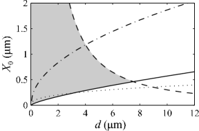
Figure 3: Stability diagram for the size $d$, and the well separation $X_{0}$. The gray area represents pairs of $d$ and $X_{0}$ for which a 1 mG fluctuation of an external magnetic field does not significantly disturb the double-well. The solid line delimits the zone where the tunneling rate fluctuates less than 10%, while the dashed line shows the area below which the fluctuations of the gravitational energy are less than 10% of the tunneling rate. In addition we show two additional constraints because of $B_{z}$: the area above the dotted line assures a $B_{z}$ large enough to avoid Majorana losses and the dash-dotted line corresponds to $B_{z}<100$ G. The device we describe in Sec. 4 operates at $d=5$ $\mu$m and $X_{0}=0.5$ $\mu$m.

4 Experimental realization of a magnetic double-well on an atom chip

As first proposed in hinds:2001 , the simplest scheme to obtain a hexapolar magnetic field on an atom chip uses two wires and an external uniform field (see Fig. 4.a). Denoting $2\,d$ the distance between the two wires, the value of the external field has to be $B_{0}=\mu_{0}\,I/(2\,\pi\,d)$. One then obtains a hexapole located at a distance $d$ from the surface of the chip. This configuration leads to a geometrical factor $\alpha=1$. In order to safely lie in the stability domain in figure 3, one can choose $d=5$ $\mu$m. This leads to a current $I=20$ mA and to a uniform magnetic field $B_{0}=8$ G. The required relative stability $\Delta B_{0}/B_{0}$ for this field is about $10^{-4}$ since fluctuations of only 1 mG are tolerable . Relative temporal stability of this magnitude can be achieved with the appropriate experimental precaution, but it is quite difficult to produce a spatially homogeneous field on the overall length of the condensate (1 mm) with such accuracy.

Figure 4: Two configurations that produce a hexapolar magnetic field. Each wire carries the same current $I$. In (a) the hexapole is obtained with two wires and a uniform magnetic field $B_{0}=\mu_{0}\,I/(2\,\pi\,d)$. In (b) it is produced by 5 wires and no external field. In the first configuration the stability of $B_{0}$ relative to $I$ is critical. The second configuration avoids this difficulty provided that the wires are connected in series.

To circumvent this difficulty we propose to realize the hexapolar field using only wires on the chip. Assuming all the wires are fabricated on the same layer, at least five wires must be used to create a hexapole. As seen in figure 4, the distance between the wires can be chosen so that a hexapole is obtained with the same current running in all the wires. This allows rejection of the noise from the power supply delivering the current $I$. For this geometry, we calculate $\alpha=4/\sqrt{3}$ which is the value we used to plot the curves in figure 3.

We have implemented this five wire scheme on an atom chip. The wires are patterned using electron beam lithography on an oxidized silicon wafer covered with a 700 nm thick evaporated gold layer. Each wire has a 700 nm$\,\times\,$700 nm cross-section and is 2 mm long. Figure 5 shows the schematic diagram of the chip and a SEM image of the wire ends. This design allows us to send the same current in the five wires using a single power supply. The extra connections are used to add a current in the central wire in order to split the hexapole into two quadrupoles without any external magnetic field. We can also change the current in the left (right) pair of wires in order to release the atoms from the left (right) trap when the separation between the wells is large enough. The transverse wires connecting the five wires at their ends insure the longitudinal confinement of the atoms in a box like potential.

The distance $d$ characterizing the wire spacing is 5 $\mu$m. Using the exact expression of the magnetic field created by the five wires, we have carried out numerical calculation of the spectrum of the double-well. Using a transverse field $b=60$ mG and a longitudinal field $B_{z}=550$ mG, we obtain a spacing between the wells of $2\,X_{0}=1.0$ $\mu$m and a tunneling rate of $\delta=2\pi\times 290$ Hz. The parameters have been chosen to fulfill the condition $\omega_{0,2}=10\,\delta$ and to lie in the center of the stability domain. We have checked numerically that the two conditions on the stability of the tunneling rate and of the gravitational energy shift are indeed fulfilled.

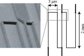
Figure 5: Schematic and SEM picture of our five wire device. The design allows one to send the same current with a single power supply in all the wires to create a magnetic hexapole. The connections on the central wires allow us to imbalance the currents between the central wire, the two left wires and the two right wires.

4.1 Splitting of a thermal cloud

In order to load the double-well with a sample of cold ⁸⁷Rb atoms, the five wire chip is glued onto an atom chip like that used in a previous experiment to produce a Bose-Einstein condensate esteve:2004 . The five wire chip surface is located approximately 150 $\mu$m above the surface of the other chip. This two-chip design allows one to combine wires having very different sizes (typically 50 $\mu$m $\times$ 10 $\mu$m for the first chip and 700 nm $\times$ 700 nm for the five wire chip) and therefore different current-carrying capacities in a single device. Large currents are needed to efficiently capture the atoms from a MOT in the magnetic trap.

Using evaporative cooling, we prepare a sample of cold atoms in a Ioffe trap created by a Z-shaped wire on the first chip and a constant external field. Transfer of the atoms to the double-well potential is achieved by ramping down the current in the Z-shaped wire and the external field while we ramp up the currents in the five wires. The final value of the current in the central wire is smaller (10.4 mA) than for the one in the other wires (17.5 mA). We use the fact that an imbalanced current in the central wire is qualitatively equivalent to adding an external transverse field to the hexapole. Ignoring the field due to the lower chip, these current values lead to two trapping minima located on the $y$-axis. The position of the upper minimum is superimposed on the position of the Ioffe trap due to the lower chip. We typically transfer of order $10^{4}$ atoms having a temperature below 1 $\mu$K.

To realize a splitting experiment, we then increase the current in the central wire to 17.5 mA and decrease the current in the other wires to 15 mA. The duration of the ramp is 20 ms. If the external transverse field is zero, the two traps located on the $y$-axis coalesce when all the currents are equal and then split along the $x$-axis when the current in the central wire is above the one in the other wires. Then, by lowering the current in the left (right) wires to zero, we eliminate the atoms in the left (right) trap and measure the number of atoms remaining in the other trap using absorption imaging. If the external magnetic field has a small component along the $y$-axis, the coalescence point is avoided and the atoms initially in the upper trap preferentially go in the right (left) trap if $b_{y}$ is positive (negative). The number of atoms in the left or in the right well as a function of $b_{y}$ is plotted in figure 6. As expected, we observe a 50% split between the two wells if the two traps coalesce using $b_{y}=0$. For an amplitude of the magnetic field $b_{y}$ larger than 0.6 G, the transferred fraction of atoms is almost zero. For this specific value of the transverse magnetic field, the atomic temperature at closest approach between the wells is estimated to be 420 nK. On the other hand, for this transverse field and for the longitudinal field $B_{z}=1$ G used in the experiment, the barrier height between wells at closest approach is 12 $\mu$K. Thus, the value of the atomic temperature seems too small to explain our observations. The estimated atomic temperature is calculated knowing the initial temperature (220 nK) and assuming adiabatic compression. We have reason to be confident in the adiabaticity because the temperature is observed to be constant when the splitting ramp is run backward and forward at $b_{y}=0.6$ G. More precisely, numerical calculations of the classical trajectories during the splitting indicate that the typical width of the curves shown on figure 6 is approximately three times too large. For the moment, we do not have a satisfactory explanation for this broadening.

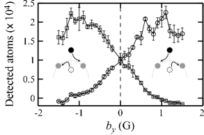
Figure 6: Final number of atoms in the right well ($\square$) and in the left well ($\circ$) after a splitting experiment. The schematics depict the trajectories of the two traps during the sequence. Initially all the atoms are in the upper trap, depending on the sign of the $y$ component of $b$, the atoms preferentially end in the left or in the right well. The minimal distance between the traps depends on the modulus of $b_{y}$. This distance is zero if $b_{y}=0$, leading to a splitting with half of the atoms in each well.

4.2 Longitudinal potential roughness

For our present setup, the actual longitudinal potential differs from the ideal box-like potential because of distortions in the current distribution inside the wires esteve:2004 ; Schumm:2005 . Preliminary measurements indicate a roughness with a rms amplitude of a few mG and a correlation length of a few $\mu$m. The condensate will thus be fragmented. Each fragment will be trapped in a potential with a typical longitudinal frequency of about 400 Hz. Given the same number of atoms and the same total length for the whole condensate, the longitudinal density in each fragment will be approximately ten times higher than for the ideal box-like potential. Thus the Rabi regime may be out of reach with our present setup. More precise measurements of the exact longitudinal potential shape are in progress to determine the maximum ratio $E_{J}/(N^{2}\,E_{C})$ we can actually achieve. Improved wire fabrication techniques may allow us to obtain a flatter longitudinal potential and to increase the $E_{J}/(N^{2}\,E_{C})$ ratio.

5 Conclusion

We have shown that atom chip based setups are well suited to produce a stable magnetic double-well potential. Our main argument is that atom chips allow one to design a current distribution having a characteristic size small enough so that oscillations of a condensate between the wells can be reproducible despite a noisy electromagnetic field environment.

We have fabricated a device using five wires spaced by a distance of a few microns. The preliminary data in Fig. 6 show that we have good control over our transverse magnetic potential, although we cannot entirely validate our design choices before having observed coherent oscillations. To do this it remains to reproducibly place a condensate in the trap so that the two mode description applies and can be tested.

This work was supported by the E.U. under grants IST-2001-38863 and MRTN-CT-2003-505032 and by the D.G.A. (03.34.033).

References

- (1) R. Folman, P. Krüger, J. Schmiedmayer, J. Denschlag, and C. Henkel, Adv. Atom. Mol. Opt. Phys. 48, 263 (2002), and references therein.
- (2) P. Treutlein, P. Hommelhoff, T. Steinmetz, T. W. Hänsch, and J. Reichel, Phys. Rev. Lett. 92, 203005 (2004).
- (3) Y.-J. Wang, D. Z. Anderson, V. M. Bright, E. A. Cornell, Q. Diot, T. Kishimoto, M. Prentiss, R. A. Saravanan, S. R. Segal, and S. Wu, cond-mat/0407689 (2004).
- (4) C. Zimmermann, Private communication (2005).
- (5) F. Dalfovo, S. Giorgini, L. Pitaevskii, and S. Stringari, Rev. Mod. Phys. 71, 463 (1999), and references therein. A. J. Legget, Rev. Mod. Phys. 73, 307 (2001), and references therein.
- (6) M. Albiez, R. Gati, J. Foelling, S. Hunsmann, M. Cristiani, and M. K. Oberthaler, cond-mat/0411757 (2005).
- (7) D. Cassettari, B. Hessmo, R. Folmann, T. Maier, and J. Schmiedmayer, Phys. Rev. Lett. 85, 5483 (2000).
- (8) E. A. Hinds, C. J. Vale, and M. G. Boshier, Phys. Rev. Lett. 86, 1462 (2001).
- (9) W. Hänsel, J. Reichel, P. Hommelhoff, and T. W. Hänsch, Phys. Rev. A 64, 063607 (2001).
- (10) E. Andersson, T. Calarco, R. Folman, M. Andersson, B. Hessmo, and J. Schmiedmayer, Phys. Rev. Lett. 88, 100401 (2002).
- (11) I. Bouchoule, physics/0502050 (2005).
- (12) V. M. Kaurov and A. B. Kuklov, Phys. Rev. A 71, 011601(R) (2005).
- (13) A. Smerzi, S. Fantoni, S. Giovanazzi, and S. R. Shenoy, Phys. Rev. Lett. 79, 4950 (1997).
- (14) S. Raghavan, A. Smerzi, and V. M. Kenkre, Phys. Rev. A 59, 620 (1999).
- (15) K. K. Likharev, Dynamics of Josephson Junctions and Circuits (Gordon and Breach Science Publishers, New York, 1986).
- (16) S. Groth, P. Krüger, S. Wildermuth, R. Folman, T. Fernholz, J. Schmiedmayer, D. Mahalu, and I. Bar-Joseph, Appl. Phys. Lett. 85, (2004).
- (17) J. Estève, C. Aussibal, T. Schumm, C. Figl, D. Mailly, I. Bouchoule, C. I. Westbrook, and A. Aspect, Phys. Rev. A 70, 043629 (2004).
- (18) T. Schumm, J. Estève, C. Figl, J.-B. Trebbia, C. Aussibal, H. Nguyen, D. Mailly, I. Bouchoule, C.I. Westbrook and A. Aspect, Eur. Phys. J. D 32, 171 (2005).