Elastic lever arm model for myosin V

Abstract

We present a mechanochemical model for myosin V, a two-headed processive motor protein. We derive the properties of a dimer from those of an individual head, which we model both with a 4-state cycle (detached, attached with ADP.Pi, attached with ADP and attached without nucleotide) and alternatively with a 5-state cycle (where the power stroke is not tightly coupled to the phosphate release). In each state the lever arm leaves the head at a different, but fixed, angle. The lever arm itself is described as an elastic rod. The chemical cycles of both heads are coordinated exclusively by the mechanical connection between the two lever arms. The model explains head coordination by showing that the lead head only binds to actin after the power stroke in the trail head and that it only undergoes its power stroke after the trail head unbinds from actin. Both models (4- and 5-state) reproduce the observed hand-over-hand motion and fit the measured force-velocity relations. The main difference between the two models concerns the load dependence of the run length, which is much weaker in the 5-state model. We show how systematic processivity measurement under varying conditions could be used to distinguish between both models and to determine the kinetic parameters.

Introduction

Myosin V is a motor protein involved in different forms of intracellular transport Reck-Peterson et al. (2000); Vale (2003). Because it was the first discovered processive motor from the myosin superfamily and due to its unique features, including a very long step size, it has drawn a lot of attention in recent years and now belongs to the best studied motor proteins. The experiments have characterized it mechanically Mehta et al. (1999); Rock et al. (2000); Rief et al. (2000); Veigel et al. (2002); Purcell et al. (2002), biochemically De La Cruz et al. (1999, 2000b, 2000a); Yengo et al. (2002); Purcell et al. (2002), optically Ali et al. (2002); Forkey et al. (2003); Yildiz et al. (2003) and structurally Walker et al. (2000); Burgess et al. (2002); Wang et al. (2003); Coureux et al. (2003). These studies have shown that myosin V walks along actin filaments in a hand-over-hand fashion Yildiz et al. (2003) with an average step size of about 35 nm, roughly corresponding to the periodicity of actin filaments Mehta et al. (1999); Rief et al. (2000); Veigel et al. (2002); Ali et al. (2002), a stall force of around 2 pN Rief et al. (2000) and a run length of a few microns Rief et al. (2000); Sakamoto et al. (2003); Baker et al. (2004). Under physiological conditions, ADP release was shown to be the time limiting step in the duty cycle De La Cruz et al. (1999); Rief et al. (2000). Two stages of the power stroke have been resolved: one about 20nm, possibly connected with the release of phosphate, and another one of 5nm, probably occurring upon release of ADP Veigel et al. (2002). Despite all this progress, the definite answer to the questions how the mechanical and the chemical cycle are coupled and how the heads communicate with each other to coordinate their activity has not yet been found.

Theoretical models for processive molecular motors can follow different goals. What most models have in common is that they identify a few long-living states in the mechanochemical cycle and assume stochastic (Markovian) transitions between them. The differences between models start in the way these states are chosen. An approach that has been applied to myosin V Kolomeisky and Fisher (2003), kinesin Peskin and Oster (1995); Schief and Howard (2001); Thomas et al. (2002), as well as to other biological mechanisms of force generation, including actin polymerization Peskin et al. (1993) and RNA polymerase Wang et al. (1998), models the motors as stochastic steppers. These models describe the whole motor as an object that can go through a certain number of conformations (typically a few) with different positions along the track. After the completion of one cycle (which is, in models for myosin V and kinesin, tightly coupled to the hydrolysis of one ATP molecule), the motor advances by one step. All steps are reversible and at loads above the stall the motor is supposed to walk backwards and thereby regenerate ATP. The approach has been particularly useful for interpreting the measured force-velocity relations and relating them to the kinetic parameters and positions of substeps Schief and Howard (2001); Fisher and Kolomeisky (2001); Kolomeisky and Fisher (2003). A limitation of such models is that they assume coordinated activity of both heads rather than explaining it. They also assume that the motor strictly follows the regular cycle and there is no place for events like steps of variable length and dissociation from the track, although the latter can be incorporated into the models by proposing a different dissociation rate for each state in the cycle.

In this Article we present a physical model for the processive motility of myosin V. The basic building block of our model is an individual head, which we model in a similar way as the models for conventional myosins do Hill (1974), albeit with different rate constants. The head is connected to the lever arm, which we model as an elastic rod, whose geometry we infer from electron microscopy studies Walker et al. (2000); Burgess et al. (2002). The two lever arms are connected through a flexible joint and this is the exclusive way of communication between them. We will derive the properties of the dimer from those of the individual head.

The Model

To describe each myosin V head we use a model based on the 4-state cycle as postulated by Lymn and Taylor (1971) and used in many quantitative muscle models Hill (1974) (Fig. 2A). We restrict ourselves to the long-living states in the cycle: detached with ADP.Pi, bound with ADP.Pi, bound with ADP, detached with ADP and bound without a nucleotide. The bound state with ATP and the free state with ATP have both been found to be very short-lived De La Cruz et al. (1999) and we therefore omit them in our description, i.e., we assume that binding of ATP to a bound head leads to immediate detachment and ATP hydrolysis. The detached state without a nucleotide is very unlikely to be occupied because of the low transition rates leading to it and we omit it from our scheme as well.

One question that has not yet been definitely answered, is whether Pi release occurs before or during the power stroke, i.e., whether a head which is mechanically restrained form conducting its power stroke can release Pi or not. The 4-state model assumes a tight linkage between the Pi release and the power stroke. While the 4-state model has been successfully applied to myosin II (e.g., Duke (1999); Vilfan and Duke (2003)), recent experimental evidence suggests that the lead head can release Pi before the power stroke Rosenfeld and Sweeney (2004). We therefore also discuss an alternative 5-state model. In the 5-state model we introduce an additional state ADP^′ in which the phosphate is already released, but the lever-arm is still in the pre-powerstroke state. The next transition, ADP release, however, is still linked to the completion of the full power-stroke. This is necessary in order to explain head coordination and also in agreement with experiments that show a strain-dependence in the ADP release rate in single-headed molecules Veigel et al. (2002). The extended duty cycle of a head is shown in Fig. 2B.

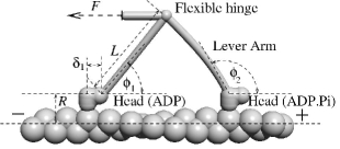
Figure 1: The myosin V dimer is modeled as two heads, each connected to a lever arm which leaves the head at a certain angle $\phi$, depending on the state of the head. The two lever arms, modeled as elastic beams, are connected with a flexible joint, which is also connected to the external load.

A)

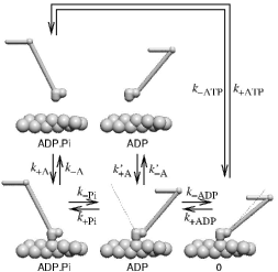
B)

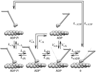
Figure 2: A) The mechanochemical cycle of each individual head. The head attaches to actin in the state with ADP and Pi bound on it, undergoes a large conformational change upon Pi release, another smaller conformational change upon ADP release, then binds ATP and enters the very weakly bound state, which dissociates quickly. B) The mechanochemical cycle in the 5-state model. In this scenario, the phosphate release and the power stroke are two separate transitions.

Table 1: Geometric parameters of a myosin V head (see also Fig. 1 for their definition).

Lever arm length	$L$	$26\,{\rm nm}$
Lever arm start	$R$	$8\,{\rm nm}$
Lever arm start	$\delta_{\rm ADP.Pi}$	$0\,{\rm nm}$
Lever arm start	$\delta_{\rm ADP,apo}$	$3.5\,{\rm nm}$
Angle ADP.Pi	$\phi_{\rm ADP.Pi}$	$115^{\circ}$
Angle ADP	$\phi_{\rm ADP}$	$50^{\circ}$
Angle apo	$\phi_{\rm apo}$	$40^{\circ}$

A head always binds to an actin subunit in the same relative position. In each state, the proximal end of the lever arm leaves the head in a fixed direction in space, determined by the polar angle $\phi$ towards the filament plus end and the azimuthal angle $\theta=\theta_{0}i$ of the actin subunit $i$ to which the head is bound. The geometry of the molecule and the angles were inferred from images obtained with electron microscopy Walker et al. (2000); Burgess et al. (2002). They are summarized in Table 1. In our calculations we assume a 13/6 periodicity of the actin helix (6 rotations per 13 subunits), which means $\theta_{0}=2\pi\times 6/13$.

We assume that the lever arm has the properties of a linear, uniform and isotropic elastic rod, described with the bending modulus $EI$. Then the local curvature $\kappa$ is determined from $M=EI{\mathbf{\kappa}}$, where $M$ is the local bending moment (torque). The lever arms from both heads are joined together (and to the tail) with a flexible joint which allows free rotation in all directions. For a certain configuration of chemical states, binding sites of both heads and a given external force, the three-dimensional shape and the bending energy of both lever arms can be calculated numerically as described in the Appendix. Some of the calculated shapes are shown in Fig. 3.

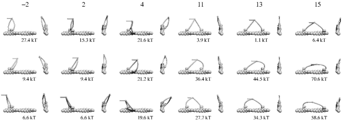
Figure 3: Calculated shapes and bending energies of dimers, bound $i$ subunits apart ($i=-2,2,\ldots,15$) and in different states: first in post-, second in the pre-powerstroke state (upper row), both in the post-powerstroke state (middle row) and both in the pre-powerstroke state (bottom row). Each configuration is shown in side and front view. If both heads are in the same state (bottom two rows) there is a significant cost in elastic energy needed to buckle one of the lever arms. Binding of the lead head before the trail head undergoes the power stroke is therefore unlikely.

We calculate the free energy of a dimer state as

$$G=G_{1}+G_{2}+U_{1}+U_{2}+Fx\;,$$ (1)

where $G_{1}$ and $G_{2}$ are the intrinsic free energies of both heads (which depend on the chemical state of the head and the concentrations of nucleotides), $U_{1}$ and $U_{2}$ are the energies stored in the elastic deformation of each lever arm, and $Fx$ is the work done against the external load ($x$ denotes the coordinate of the flexible joint along the filament axis with positive values towards the plus end, while positive values of $F$ denote a force pulling towards the minus end, against the direction of motion of an unloaded motor).

Transition rates

There are two exact statements we can make about the kinetic rates of the duty cycle that follow from the principle of detailed balance. The first statement relates the forward and the backward rate of any reaction to the free energy difference between the initial and the final state. For any transition the principle of detailed balance states that

$$\frac{k_{+i}}{k_{-i}}=\frac{k^{0}_{+i}}{k^{0}_{-i}}e^{-\frac{\Delta U+F\Delta x}{k_{B}T}}$$ (2)

where $\Delta U$ denotes the change in elastic energy of the dimer and $F\Delta x$ the work performed against the external load.

The second exact statement can be derived by multiplying together the detailed balance conditions for a monomer in the absence of any external force along a closed pathway in Fig. 2. After one cycle the free energy of the bound monomeric head returns to its initial value, while the total free energy change in the system equals the amount gained from the hydrolysis of one ATP molecule. The resulting relation reads

$$\frac{k^{0}_{\rm+A}k^{0}_{\rm-Pi}k^{0}_{\rm-ADP}k_{\rm+ATP}[{\rm ATP}]}{k_{\rm-A}k^{0}_{\rm+Pi}[{\rm Pi}]k^{0}_{\rm+ADP}[{\rm ADP}]k^{0}_{\rm-ATP}}\\ =e^{\frac{\Delta G_{ATP}}{k_{B}T}}=e^{\frac{\Delta G^{0}}{k_{B}T}}\frac{[{\rm ATP}]}{[{\rm ADP}][{\rm Pi}]}$$ (3)

and provides an important constraint on the kinetic rates of the model. In the 5-state model, we obtain an equivalent equation,

$$\frac{k^{0}_{\rm+A}k^{0}_{\rm-Pi}k^{0}_{\rm+PS}k^{0}_{\rm-ADP}k_{\rm+ATP}[{\rm ATP}]}{k_{\rm-A}k^{0}_{\rm+Pi}[{\rm Pi}]k^{0}_{\rm-PS}k^{0}_{\rm+ADP}[{\rm ADP}]k^{0}_{\rm-ATP}}\\ =e^{\frac{\Delta G^{0}}{k_{B}T}}\frac{[{\rm ATP}]}{[{\rm ADP}][{\rm Pi}]}\;.$$ (4)

A similar statement also holds for the rates along the inner loop in the reaction scheme, which involves attachment, power stroke and detachment, all in the ADP state. Because we assume that the detachment rate in the pre-powerstroke and the post-powerstroke state are both the same ($k^{\prime}_{\rm-A}$), the relation reads

$$\frac{k^{0\prime\prime}_{\rm+A}k^{0}_{\rm+PS}}{k^{0\prime}_{\rm+A}k^{0}_{\rm-PS}}=1\;.$$ (5)

When it comes to the actual force dependence of transition rates we have to rely on approximations. An approach that is most widely used when modeling motor proteins, but also other conformational changes, like the gating of ion channels, involves the Arrhenius theory of reaction rates Hill (1974). It proposes that the protein has to reach an activation point ($x_{a}$) somewhere between the initial ($x_{i}$) and the final state ($x_{f}$) by thermal diffusion, but completes the reaction rapidly after that. Therefore, the force dependence of the forward rate can be modeled as

$$k_{+i}=k_{+i}^{0}e^{-\frac{U(x_{a})-U(x_{i})}{k_{B}T}}\qquad k_{-i}=k_{-i}^{0}e^{-\frac{U(x_{a})-U(x_{f})}{k_{B}T}}$$ (6)

where $U(x)$ means the total potential (bending of both lever-arms and work done against the external load) which a head has to overcome to bring the lever arm angle into a given state. We use the variable $\epsilon$ to denote the relative position of the activation point between the initial and the final state, so that $x_{a}=(1-\epsilon)x_{i}+\epsilon x_{f}$. Unless otherwise noted, we will assume $\epsilon=0.5$. Not precisely identical, but useful for practical purposes is also the approximation $U(x_{a})=(1-\epsilon)U(x_{i})+\epsilon U(x_{f})$. Therefore we get the following expression for the force-dependence of the transition rate:

$$k_{+i}=k_{+i}^{0}e^{\frac{\epsilon\Delta U}{k_{B}T}}$$ (7)

For reactions that involve the binding and unbinding of a head, Eq. 2 is valid, but one expects the activation point to be much closer to the bound state. The strain-dependence of the detachment rate for heads in the ADP and ATP.Pi state has not yet been measured and we therefore neglect it, assuming that the detachment rate is force-independent, $k_{\rm-A}\equiv k_{\rm-A}^{0}$. The attachment rate then relates to the potential difference as

$$k_{\rm+A}=k_{\rm+A}^{0}e^{-\frac{\Delta U}{k_{B}T}}\;.$$ (8)

Choice of kinetic parameters

Table 2: Kinetic parameters of the model

Parameter		Value		Source
		4-state	5-state
$k^{0}_{\rm+A}$	actin binding with ADP.Pi	$5000\,{\rm s^{-1}}$	$5000\,{\rm s^{-1}}$	est. from run length
$k_{\rm-A}$	actin release with ADP.Pi	$1\,{\rm s^{-1}}$	$50\,{\rm s^{-1}}$	est. from run length
$k^{0\prime}_{\rm+A}$	actin binding with ADP	$5000\,{\rm s^{-1}}$	$5000\,{\rm s^{-1}}$	$\approx k^{0}_{\rm+A}$ De La Cruz et al. (1999)
$k^{\prime}_{\rm-A}$	actin release with ADP	$0.1\,{\rm s^{-1}}$	$0.1\,{\rm s^{-1}}$	$0.032\,{\rm s^{-1}}$ De La Cruz et al. (1999), $1.1\,{\rm s^{-1}}$ Baker et al. (2004)
$k^{0}_{\rm-Pi}$	Pi release	$200\,{\rm s}^{-1}$	$200\,{\rm s}^{-1}$	$>250\,{\rm s}^{-1}$ De La Cruz et al. (1999), $110\,{\rm s}^{-1}$ Yengo and Sweeney (2004), $228\,{\rm s}^{-1}$ Rosenfeld and Sweeney (2004)
$\epsilon_{\rm-Pi}$	activation point	$0.3$	–	F-v relation at high loads
$k^{0}_{\rm+Pi}$	Pi binding	$10^{-4}\,{\mu\rm M}^{-1}{\rm s}^{-1}$	$10^{-2}\,{\mu\rm M}^{-1}{\rm s}^{-1}$	guess
$k^{0}_{\rm+PS}$	power stroke	–	$10^{4}\,{\rm s}^{-1}$	guess
$k^{0}_{\rm-PS}$	reverse stroke	–	$0.05\,{\rm s}^{-1}$	$k^{0}_{\rm+PS}/k^{0}_{\rm-PS}$ from the stall force
$k^{0}_{\rm-ADP}$	ADP release	$20\,{\rm s}^{-1}$	$20\,{\rm s}^{-1}$	$k_{\rm-ADP}=13\,{\rm s}^{-1}$ for dimers Rief et al. (2000)
$k^{0}_{\rm+ADP}$	ADP binding	$12\,{\mu\rm M}^{-1}{\rm s}^{-1}$	$12\,{\mu\rm M}^{-1}{\rm s}^{-1}$	$12.6\,{\mu\rm M}^{-1}{\rm s}^{-1}$ De La Cruz et al. (1999), $14\,{\mu\rm M}^{-1}{\rm s}^{-1}$ Wang et al. (2000)
$k_{\rm+ATP}$	ATP binding, actin release	$0.7\,{\mu\rm M}^{-1}{\rm s}^{-1}$	$0.7\,{\mu\rm M}^{-1}{\rm s}^{-1}$	$0.9\,{\mu\rm M}^{-1}{\rm s}^{-1}$ De La Cruz et al. (1999); Rief et al. (2000), $0.6-1.5\,{\mu\rm M}^{-1}{\rm s}^{-1}$ Veigel et al. (2002)
$k^{0}_{\rm-ATP}$	actin binding with ATP release	$0.07\,{\rm s}^{-1}$	$1.2\,{\rm s}^{-1}$	Eq. 3, Eq. 4

Some of the transition rates in the cycle are well known from the literature. $k_{\rm-ADP}$ is the limiting rate both for running myosin V molecules and for single-headed constructs at low ATP concentrations. The measured values are $13\,{\rm s}^{-1}$ Rief et al. (2000) for dimers and $12\,{\rm s}^{-1}$ De La Cruz et al. (1999), $13$–$22\,{\rm s^{-1}}$ Trybus et al. (1999), and $4.5$–$7\,{\rm s}^{-1}$ Molloy and Veigel (2003) for monomers. Because the actual rate in a dimer is slowed down as compared to the monomer, we use the value $k^{0}_{\rm-ADP}=20\,{\rm s}^{-1}$. The reverse rate, $k_{\rm+ADP}$ can be determined from the inhibitory effect of ADP on the velocity and has been estimated as $12.6\,{\rm\mu M}^{-1}{\rm s}^{-1}$ De La Cruz et al. (1999), $4.5\,{\rm\mu M}^{-1}{\rm s}^{-1}$ Rief et al. (2000), $14\,{\rm\mu M}^{-1}{\rm s}^{-1}$ Wang et al. (2000).

Equally well known is the rate for ATP binding, $k_{\rm+ATP}$, which has been measured as $0.9\,{\rm\mu M}^{-1}{\rm s}^{-1}$ De La Cruz et al. (1999); Rief et al. (2000), $0.6$–$1.5\,{\rm\mu M}^{-1}{\rm s}^{-1}$ Veigel et al. (2002). For the Pi release rate the estimates range from $k_{\rm-Pi}>250\,{\rm s}^{-1}$ De La Cruz et al. (1999) to $110\,{\rm s}^{-1}$ Yengo and Sweeney (2004). We therefore use the value $k_{\rm-Pi}=200\,{\rm s}^{-1}$.

There is some more discrepancy between the current values for the release rate from actin in the ADP state. While direct measurements gave $k^{\prime}_{-\rm A}=0.032\,{\rm s}^{-1}$ De La Cruz et al. (1999) and $0.08\,{\rm s}^{-1}$ Yengo and Sweeney (2004), a recent estimate from the run length led to a higher value of $1.1\,{\rm s}^{-1}$ Baker et al. (2004). We use an intermediate value of $k^{\prime}_{-\rm A}=0.1\,{\rm s}^{-1}$. For the attachment rate in the ADP state, we set $k^{0\prime}_{+\rm A}\approx k^{0}_{+\rm A}$, based on kinetic measurements De La Cruz et al. (1999).

This leaves us with a total of 4 unknown kinetic rates, of which 3 need to be estimated from the measured stepping behavior and run length data, while one can be determined from Eq. 3.

Results

Choice of the value for the bending modulus

There are two ways to estimate the bending stiffness of the myosin V lever arm - one from its structure and analogy with similar molecules and the other one from the observed behavior of the dimeric molecule. The lever arm consists of 6 IQ motifs, forming an $\alpha$-helix, surrounded by 6 calmodulin or other light chains Wang et al. (2003); Terrak et al. (2003). One possible estimate for the stiffness of the lever arm can be obtained by approximating it with a coiled-coil domain, as has been done by Howard and Spudich (1996). Generally, the stiffness of a semiflexible molecule is related to its persistence length $\ell_{p}$ as $EI=\ell_{p}k_{B}T$. Howard and Spudich estimated the persistence length of a coiled-coil domain as $100\,{\rm nm}$, which yields $EI\approx 400\,{\rm pN\,nm}^{2}$. Other researchers report values of $\ell_{p}=130\,{\rm nm}$ for myosin Hvidt et al. (1982) and $\ell_{p}=150\,{\rm nm}$ for tropomyosin Swenson and Stellwagen (1989); Phillips and Chacko (1996).

On the other hand, we can estimate the stiffness from the force a lever arm has to bear under conditions close to stall. We do this by calculating the distribution of binding probabilities to different sites at $F=1.8\,{\rm pN}$, which is close to stall force. We assume that the binding rate to each site is proportional to its Boltzmann weight, $\exp(-G/k_{B}T)$, which is equivalent to assuming that the activation point of the binding process is close to the final state and that the reverse reaction (detachment in the state with ADP.Pi) has no force-dependence in its rate. The expectation value of the binding position of the lead head relative to the trail head is shown in Fig. 4. It shows that a stiffness of $EI\gtrsim 1000\,{\rm pN\,nm^{2}}$ is necessary to allow stepping at loads of this magnitude.

Figure 4: The average step size under a load of $F=1.8\,{\rm pN}$ as a function of the lever arm elasticity $EI$. The step size was calculated from attachment probabilities of the lead head (ADP.Pi state) relative to the bound trail head (ADP state).

For these reasons, we use the value $EI=1500\,{\rm pN\,nm^{2}}$. This corresponds to an elastic constant (measured at the joint) of

$$k=3EI/L^{3}=0.25\,{\rm pN/nm}\;.$$ (9)

The elastic constant for longitudinal forces (with respect to the lever arm) is much higher. If we approximate the lever arm with a homogeneous cylinder of radius $r=1\,{\rm nm}$, we can estimate it as $k_{L}=4EI/(r^{2}L)=230\,{\rm pN/nm}$. We therefore neglect the longitudinal extensibility of the lever arm in all calculations.

A similar value ($EI=1300\,{\rm pN\,nm^{2}}$) has also been obtained by analyzing data from optical trap experiments on single-headed myosin V molecules with different lever arm lengths Moore et al. (2004). Even though it is somewhat larger (about 3 times) than the values estimated for myosin II (Howard and Spudich, 1996), there is no solid evidence that the structures with different light chains have the same bending stiffness. On the other hand, there could have been some evolutionary pressure to increase the lever arm stiffness, as it is directly related to the stall force of myosin V. While we are not able to give a definite answer to the question whether the lever arm behaves like a uniform elastic rod or whether there is a pliant region close to the head, we favor the first hypothesis because the estimated lever arm elasticity already is more than sufficient to explain the mechanical properties of the dimeric molecule.

Step size distribution

Figure 3 shows the energies stored in the elastic distortions of the lever arms of both heads in the pre-powerstroke or the post-powerstroke state. For example, if the first head is in the ADP.Pi state and the second head binds before the first one undergoes a power stroke, this is connected with an energy cost of $6.6\,k_{B}T$. The attachment rate of the lead head before the power stroke in the trail head is therefore more than 100 times slower than after the power stroke.

Because the lead head normally attaches to actin while the trail head is in the ADP state, we can determine the probability that the lead head binds to an actin site $i$ subunits in front of the trail head from the Boltzmann factors formed from the bending energy in the final configuration, $P_{i}\propto\exp(-(U_{1}+U_{2})/k_{B}T)$. Here $U_{1}+U_{2}$ denotes the sum of elastic energies stored in both lever arms if the trail head is in the ADP state and the lead head in the ADP.Pi state, bound $i$ sites in front of the trail head. The resulting distributions for different lever arm lengths are shown in Fig. 5. For the lever arm consisting of 6 IQ motifs, the result is a mixture of 11 and 13 subunit steps, whereby 13 subunits dominate. Azimuthal distortion plays a major role in the bending energy, therefore binding is only likely to sites 2, 11, 13 and 15, on which the azimuthal angles of both heads differ by not more than $27^{\circ}$.

Figure 5: Step size distribution for 4 different lever arm lengths L: 10nm (2IQ), 18nm (4IQ), 26nm (6IQ) and 34nm (8IQ) and no external load. The histograms show the probability that a lead head (ADP.Pi state) will bind $i$ sites in front of the trail head in the post-powerstroke ADP state. The probabilities were determined from the Boltzmann factors, resulting from the elastic distortion energy of the configuration. Azimuthal distortion plays a crucial role role in determining the step size, which is the reason why the binding is always concentrated on sites 2, 11, 13 and 15. Taking into account the fluctuations in the actin would lead to a broader distribution, in better agreement with experiments (Walker et al., 2000).

The gated step in the cycle

A question that has been a subject of intense discussion is which step in the cycle is deciding for the coordination of the two heads. A currently often favored hypothesis proposes that the lead head undergoes its power stroke immediately after binding, thereby storing energy into elastic deformation of its lever arm and releasing it after the unbinding of the trail head. An alternative hypothesis proposes that the release of the rear head is necessary for the power stroke in the front head. As we will show below, our model favors this picture. In the 4-state scenario, this implies that the lead head is waiting in the ADP.Pi. In the 5-state scenario it is in the ADP^′ state (the pre-powerstroke ADP state). The trail head spends most of its cycle in the ADP state in both scenarios at saturating ADP concentrations.

Because this model challenges the currently prevailing view, we should first critically review the arguments supporting it. One argument includes the direct observation of telemark-shaped molecules, with the leading head leaning forward and then the lever arm tilted strongly backwards Walker et al. (2000). A more detailed image analysis, however, showed that the converter of the leading head is in the pre-powerstroke state Burgess et al. (2002). Another piece of evidence comes from experiments by Forkey et al. (2003) which show a fraction of tags on the lever arm (30-50%) that do not tilt while moving, but again the data provide no conclusive proof because the method does not allow detection of tilts symmetric with respect to the vertical axis. To conclude, one cannot say that the present experimental evidence excludes any of the two hypotheses about the moment of phosphate release and of the power stroke.

From the theoretical side, we will argue that in a model with linear elasticity the mechanism with immediate power stroke in the lead head cannot work under loads for which the motor is known to be operational. It is known that the monomeric constructs of myosin V undergo a normal duty cycle De La Cruz et al. (1999); Yengo et al. (2002), which means that no step in the cycle requires mechanical work from the outside for its completion (which would be, for example, the case if the head needed to be pulled away from actin to complete the cycle). This excludes the possibility that the free energy gain connected with binding and the power stroke exceeds $\Delta G_{\rm ATP}=100\,{\rm pNnm}$, the total available energy for one cycle. Because this and other transitions in the cycle need to be forward-running, we use the still conservative estimate that the free energy gain from binding and the power stroke cannot exceed $80\,{\rm pNnm}$. On the other hand, we can estimate the free energy that would be necessary for a head to bind to a site 13 units ahead and then undergo a conformational change. The amount of energy needed to bring the dimer into the hypothetical state with both heads in the post-powerstroke state and a strong distortion, especially of the leading lever arm, is plotted in Fig. 6. The calculation shows that the binding of the front head with the subsequent power stroke before the rear head detaches (for a load of $F=1.8\,{\rm pN}$) is only possible for values of $EI\lesssim 450\,{\rm pN\,nm^{2}}$, which is inconsistent with the lower estimate based on the observed step size (Fig. 4). Of course, we cannot rule out that there is some additional state in the middle of the power stroke which is occupied immediately while the lead head waits for the trail head to detach. But within the scope of the geometrical model with a single power stroke connected with the Pi release, we consider the scenario where the lead head instantaneously undergoes the power stroke without waiting for the detachment of the trail head unrealistic.

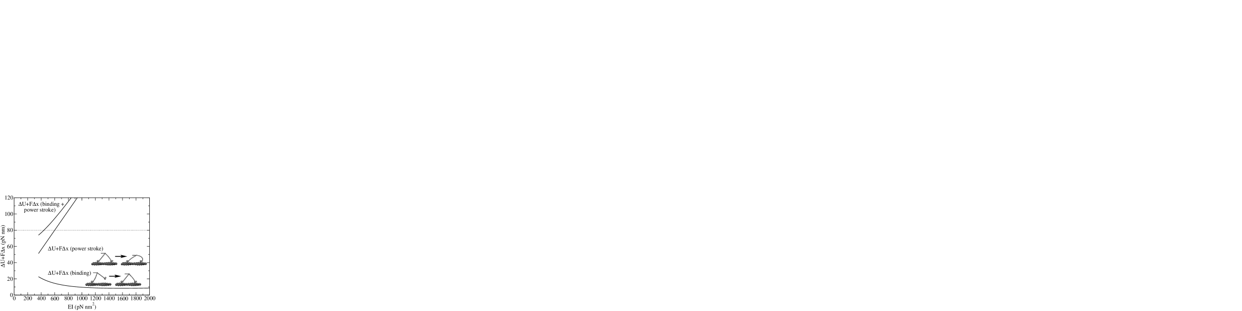
Figure 6: The amount of energy needed for the binding of the lead head and the subsequent power-stroke, plotted against the lever arm elasticity. The load pulling on the tail is $F=1.8\,{\rm pN}$. The lower curve shows the energy needed to pull the external load and distort the lever arms in order to bind the new lead head 13 sites in front of the trailing head. Note that most of this work will be performed by Brownian motion, but the potential well in the bound state still has to be strong enough to stabilize the bound state. The middle curve shows the energy needed mainly for the distortion of the lever arms when the lead head undergoes a power-stroke before the trailing head detaches. Since the sum of both cannot be higher than $80\,{\rm pN\,nm}$, we estimate that this hypothetical scenario would only be possible if the lever arm stiffness was $EI\lesssim 450\,{\rm pN\,nm^{2}}$. This is inconsistent with other requirements of the model, so we rule this scenario out.

Hidden power strokes in the dimer configuration

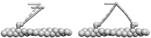
Figure 7: For a single head, the $x$-component of the power-stroke upon ADP release equals 3.3nm (for zero load). In the dimer with both heads bound, only 0.07nm of that power stroke reach the load. As a consequence, the load-dependence of transition rates between states with both heads bound is negligible.

An immediate consequence of the elastic lever arm model is that the tail position is mainly determined by the geometry of the triangle and less by the conformations of individual heads. For a monomeric head or a dimer bound by a single head, the power-stroke upon ADP release has an $x$-component (in the direction of the actin filament) of about $3.3\,{\rm nm}$ (Fig. 7). If the lead head is attached, however, the power stroke as measured on the tail is reduced by about a factor of 50. The tail movement is also closely related to the force-dependence of transition rates, which means that transitions between states with both heads bound do not show any significant load dependence. In the kinetic scheme we use here this implies that the rates of ADP release and ATP binding (the two rate limiting steps at low or forward loads) are both constant, in agreement with the flat F-v curve measured by Mehta et al. (1999).

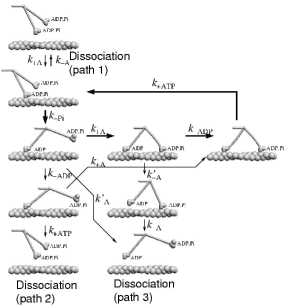
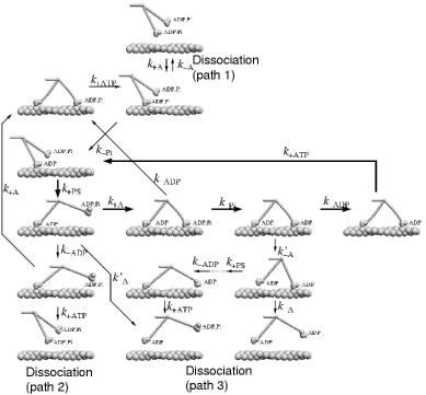
A)	B)

Figure 8: Most probable kinetic pathways for a dimer in the 4-state (A) and in the 5-state model (B). The thick arrows denote the regular pathway and the thin arrows side branches that can result in dissociation from actin. Note that the simulation was not restricted to the pathways shown here, but included all possible combinations of transitions between monomer states.

A)

B)

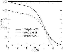
Figure 9: A) Force-velocity curves in the 4-state model, obtained from a stochastic simulation. The solid curve shows the values for $1000\mu\rm M$ ATP and the dashed curve for $1\mu\rm M$ ATP. Both curves are compared with the prediction of the simplified analytical expression (Eq. 13), dotted lines. The minor deviation is mainly due to cycles taking other pathways, neglected force-dependence of the ADP release rate and variation in the step size. Note that the velocities above $\sim 2.5\,{\rm pN}$ are not well defined because the dissociation time becomes comparable with the step time. B) Inhibition by ADP and Pi. The force-velocity relation with 1mM ATP is shown by the continuous line. The dashed line shows the same relation with additional $10\mu{\rm M}$ ADP and the dotted line with 1mM phosphate. The velocity reduction through ADP occurs at low or negative loads, while the inhibition by Pi only becomes significant close to stall conditions.

Figure 10: Force-velocity relation of the 5-state model with 1mM ATP (solid), 1mM ATP+ 10$\mu$M ADP (dashed) and 1$\mu$M ATP (dotted). Note the sharper drop at high loads as compared to the 4-state coupled model (Fig. 9).

Force-velocity and run length curves

The bending energies, calculated for each possible dimer configuration, and the transition rates were fed into a kinetic simulation to determine the average velocity of a dimeric motor and its dissociation rate from actin. The most probable kinetic pathway of the dimer is indicated by thick arrows in Fig. 8, while the thin arrows indicate some of the possible side branches that can lead to dissociation. Figure 9 shows the resulting force-velocity curves and Fig. 11 the dissociation rates.

An analytical solution of the 4-state model would, in theory, require solving the occupation probabilities for a system with about $6+8\times 3\times 3=78$ states (6 states with one head bound, plus configurations with both heads bound, where each head can occupy 3 different states and the relative positions of both heads can have 8 different values). Such a system could easily be solved numerically, but would be too complex for obtaining an insightful analytical expression. However, we will show that a simplified pathway can already lead to expressions that agree reasonably well with simulation data and are therefore useful for fitting model parameters to experimental data.

In the following, we give approximate expressions for the most significant steps in the mechanochemical cycle. The average time it takes for a head in the state 0 to bind an ATP molecule can be estimated as

$$\left<t_{\rm+ATP}\right>=\frac{1}{k_{\rm+ATP}[{\rm ATP}]}\left(1+\frac{k_{\rm+ADP}[{\rm ADP}]}{k_{-\rm ADP}}\right)$$ (10)

where the second term takes into account a reduction of the forward rate due to ADP rebinding. The second rate limiting process (especially at hight loads) is the release of phosphate. The average dwell time in the state with one head free and the other one in the ADP.Pi state is

$$\left<t_{\rm-Pi}\right>=\frac{1}{k_{\rm-Pi}}$$ (11)

The third rate limiting step is the ADP release, with the time constant

$$\left<t_{\rm-ADP}\right>=\frac{1}{k_{\rm-ADP}}\;.$$ (12)

With these three average dwell times, the motor velocity can be calculated as

$$v=\frac{\left<d\right>}{\left<t_{\rm-Pi}\right>+\left<t_{\rm-ADP}\right>+\left<t_{\rm+ATP}\right>}\;,$$ (13)

where $\left<d\right>$ denotes the average step size, which is about $35\,{\rm nm}$. The individual rates that appear in this expression can be estimated as follows: $k_{\rm-Pi}\approx k_{\rm-Pi}^{0}\exp(-F\epsilon_{\rm-Pi}d_{\rm PS}/k_{B}T)$ with $d_{\rm PS}=L(\cos\phi_{\rm ADP}-\cos\phi_{\rm ADP.Pi})+\delta$ and $k_{\rm-ADP}\approx k_{\rm-ADP}^{0}\exp(-\Delta U_{\rm-ADP}/2k_{B}T)\approx 0.65k_{\rm-ADP}^{0}$. The results for two different ATP concentrations are shown in Fig. 9A and compared with a simulation result. The analytical expression reproduces the simulation result well, with a small deviation being mainly the result of alternative pathways, neglected force-dependence of the ADP release rate and variation in the step size. The experimentally measured force-velocity curves (Mehta et al., 1999; Uemura et al., 2004) are also well reproduced, although the experiments show a more abrupt drop in velocity at high loads, with no measurable effect up to about 1pN.

In the 5-state model the power-stroke can be fast and reversible, in which case the pre- and the post-powerstroke state can reach an equilibrium and the limiting rate is proportional to the probability of the post-powerstroke state $1/(1+\exp(Fd_{\rm PS}/k_{B}T))$ - a significantly sharper load dependence than the 4-state model (Fig. 10).

Inhibition by ADP and phosphate

It is a well established observation that ADP can slow down myosin V by binding to heads in the state with no nucleotide and thereby preventing them from accepting an ATP molecule. The rate of ADP rebinding is already taken into account in the kinetic constants and the model naturally reproduces the observed behavior, as shown in Figs. 9 and 12 for the 4-state model and in Fig. 10 for the 5-state model. Not yet experimentally investigated has been the inhibition by phosphate. Its intensity depends on the reverse power-stroke rate, which is one of the open parameters of our model. In the 4-state model, Pi re-binding is necessary for the reverse power stroke and therefore some inhibition effect can be expected at high loads. The simulation shows clearly that the phosphate concentration has no effect on zero-load velocity, but it does slow down the motor close to stall (Fig. 9B). A similar effect of Pi on isometric force has also been observed in muscle Cooke and Pate (1985). In the 5-state model Pi rebinding is not mechanically sensitive and its effect is roughly force-independent. However, with the parameters chosen here, it is negligible.

Three dissociation pathways

As we can see from the kinetic scheme (Fig. 8), there are three significant pathways in the cycle that can lead to the dissociation of the myosin V dimer from an actin filament. The first pathway leaves the cycle if a dimer bound with one head in the ADP.Pi state detaches before the second head can attach. The second pathway runs through a state in which the bound head releases ADP and binds a new ATP molecule before the free head can bind. With the third pathway we denote all processes that involve the detachment of a head in the ADP state. This is the pathway favored by recent results of Baker et al. (2004). Figure 11 shows the dissociation rate, separated by contributions of the three pathways. They have the following characteristics:

Pathway 1: With this pathway we denote the dissociation of a head in the ADP.Pi state. Because this state is long-lived at high loads in the 4-state, but short-lived in the 5-state model, the resulting force-dependence of the dissociation rate differs significantly in both scenarios. In the 4-state model, the contribution to the dissociation probability per step shows a strong load-dependence, but no significant dependence on the ATP concentration. It can be estimated as

$$P_{\rm diss}\approx\frac{k_{\rm-A}}{k_{\rm-Pi}}\approx\frac{k_{\rm-A}}{k^{0}_{\rm-Pi}}e^{\frac{F\epsilon_{\rm-Pi}d_{\rm PS}}{k_{B}T}}$$ (14)

with $d_{\rm PS}=L(\cos\phi_{\rm ADP}-\cos\phi_{\rm ADP.Pi})+\delta$. The dissociation rate is higher for positive loads. From the estimated run length at $1\,{\rm pN}$ load and saturating ATP concentration of about 15 steps Clemen et al. (2003), we can estimate the unbinding rate as $k_{\rm-A}\approx 1\,{\rm s}^{-1}$. In order to account for reported run lengths of over 50 steps at low loads, we tentatively assign $k_{\rm+A}^{0}\approx 5000\,{\rm s}^{-1}$.

In the 5-state model, the situation is reversed. There the dissociation process on path 1 takes place if the trail head releases ADP before the lead head releases Pi, which can happen in two different ways: on one the rate is approximately force-independent, on the other it grows with negative (forward) loads. In order to obtain a significant contribution to the detachment rate on this pathway, we choose a higher detachment rate $k_{-A}$ than in the 4-state model ($50\,{\rm s}^{-1}$ instead of $1\,{\rm s}^{-1}$).

Pathway 2: Because the process of unbinding requires an ATP molecule, the per-step dissociation rate grows with the ATP concentration. In addition, it is proportional to the ratio of the $ADP$ dissociation rate and the actin binding rate, $k_{\rm-ADP}/k_{\rm+A}$, which is higher for negative (forward) loads. This holds in both the 4- and the 5-state scenario.

Pathway 3: The dissociation probability on pathway 3 is proportional to the detachment rate in the ADP state, $k^{\prime}_{\rm-A}$. Of all three pathways, this one shows the weakest load-dependence, although it is higher for forward loads.

We expect that systematic data on mean run length as a function of load and nucleotide concentrations will be helpful to determine the remaining model parameters.

Figure 11: Dissociation rate of myosin V dimers from actin under a high (top) and a low (bottom) ATP concentration (4-state model). The continuous line shows the total dissociation rate, the dashed line the dissociation via pathway 1, the dot-dashed line via pathway 2 and the dotted line via pathway 3.

Figure 12: Velocity (continuous, left scale) and mean run length (dashed, right scale) as a function of ADP concentration in the 4-state model for zero load and 1mM ATP.

Figure 13: Force-dependence of the dissociation rate in the 5-state model. The load dependence for positive loads is much weaker than in the 4-state model (Fig. 11)

Reverse stepping in the 5-state model

As a consequence of both the reversibility of the power stroke and the slower dissociation rate at high loads, the motor can step backwards under loads exceeding the stall force (Fig. 14). Note that these steps are not the simple reversal of forward steps (which would involve ATP synthesis), but rather indicate a different pathway in the kinetic scheme, in which both heads stay in the ADP state and alternately release actin at the leading position and rebind at the trailing. The time scale of reverse stepping is determined by the dissociation rate of a head in the ADP state, $k^{\prime}_{\rm-A}$, which we chose as $0.1\,{\rm s}^{-1}$. With a higher value of $k^{\prime}_{\rm-A}$, especially for the pre-powerstroke state (so far we assumed that the rate is equal in both ADP states), faster stepping would also be possible, although there is an upper limit on $k^{\prime}_{\rm-A}$, imposed by the dissociation rate on pathway 3.

Figure 14: Reverse stepping in the 5-state model under a high load (4.5pN), $10\,{\mu\rm M}$ ATP and $1\,{\mu\rm M}$ ADP. There is also some creeping motion between the steps, which results from the attachment and detachment of the two heads on neighboring sites, and only takes place if myosin V is allowed to follow a helical path on actin. If binding is constrained to one side of the actin filament (like on a coverslip), then only regular reverse steps with the periodicity of the helix are observed (not shown).

Discussion

We used the geometrical data of the myosin V molecule as obtained from EM images to calculate the conformations and elastic energies in all dimer configurations. These data were first used in a model with a four-state cycle and subsequently in a five-state model.

The first result, which follows directly from the bending potentials and is independent of the underlying cycle is that the elastic lever arm model explains two key components of the coordination between heads: why the lead head does not bind to actin before the power stroke in the trail head and why it does not undergo its power stroke before the trail head detaches. It also allows us to calculate the distribution of step sizes. The results for different lever-arm lengths (Fig. 5) give realistic values, in agreement with step size and helicity measurements Purcell et al. (2002); Ali et al. (2002), even though they have a slight tendency towards underestimation and also show a narrower distribution than direct electron microscopy observations Walker et al. (2000). A possible explanation for the broader distribution than predicted by the model lies in the fact that in reality the actin structure does not follow the perfect helix, as assumed in our model, but has angular deviations of up to $10^{\circ}$ per subunit Egelman et al. (1982). Taking these fluctuations into account would clearly broaden the distribution of our step sizes, but alone it cannot explain the tendency towards longer steps. The most straightforward explanation for the longer steps is that the power stroke has an additional right-handed azimuthal component. Then the configuration with the lowest energy is reached if the lead head is twisted to the right relatively to the trail head, which is the case if it is bound further away along the helix. The observation that the actin repeat is often somewhat longer than 13 subunits (some results suggest a structure closer to a 28/13 helix (Egelman et al., 1982)) could also partially explain the deviation.

An issue that has been much discussed is the contribution of Brownian motion and the power stroke to the total step size. With the geometric data used in this study, the power stroke, i.e., the distance of the lever arm tip movement between the states ADP.Pi and ADP, is about 31nm, or 5nm less than the average step size. Note that the second, smaller power stroke connected with ADP release does not contribute to the step size because it is normally followed by the detachment of the same head. Its function could be suppressing premature dissociation before the lead head binds and thus improving the processivity. The remaining 5nm can be overcome by Brownian motion before the lead head binds. However, at low loads, the binding of the lead head does not move the load, but rather stores the energy into bent lever arms. This energy gets released when the rear head detaches, which leads to an elastic power stroke immediately preceding the power stroke upon Pi release. At higher loads the situation is different, because the 5nm load movement occurs when the lead head binds. In neither case we expect the 5nm power stroke to be resolvable under normal conditions because it always immediately precedes or follows the large power stroke. However, it is possible that the substeps become observable in the presence of chemicals that slow down the power stroke (Uemura et al., 2004).

In order to fully reproduce the substeps as reported by Uemura et al. (2004), some modifications would be necessary to the model. First, part of the power-stroke would have to occur immediately upon Pi release, resulting in a lever arm move of about $12\,\rm nm$ (first substep). This step would need a very strong force-dependence in its transition rate (activation point near the final state). The subsequent longer power stroke (ADP’$\to$ADP) would then need a slower rate ($\sim 200\,\rm s^{-1}$) with less force dependence (activation point close to the initial state). However, the finding that the substep position is independent of force remains difficult to explain, because the substep involves transition between a stiff configuration, bound on both heads, and a more compliant state, bound on a single head.

The main value of both models (4- and 5-state) is that they provide a quantitative explanation of the coordinated head-over-head motility of the dimeric molecule while using only the properties of a single head as input. Both models also explain the observed force-velocity curves at high and low ATP concentration and the effect of additional ADP, but these features already reveal some testable differences between the two scenarios. One of them is the shape of the force-velocity curve. In the 4-state scenario the reverse power-stroke needs the rebinding of a phosphate molecule. This makes the cutoff behavior at high loads dependent on the Pi concentration: the velocity drop is more gradual at low, but might become sharper at high Pi concentrations (Fig. 9B). In the 5-state scenario the velocity decline is more abrupt regardless of the Pi concentration. This is the first suggestion how experiments with improved precision and a wider range of chemical conditions could help distinguishing between the two scenarios.

The main difference between the two scenarios is the predicted shape of the run length. Because the dissociation can take place on three different pathways, its rate depends on a number of parameters, of which a few cannot yet be determined by other methods. In the 4-state model the dissociation rate at high loads is dominated by detachment of a head in the ADP.Pi state and it therefore depends on the ratio $k^{0}_{\rm-A}/k^{0}_{\rm-Pi}$ (Eq. 14). A strong increase with the load is characteristic for the 4-state model, because the load slows down the phosphate release and prolongs the dwell time in the state that is most vulnerable to dissociation. Dissociation at negative (forward) loads is dominated by pathways 2 (ATP mediated actin release in one head before the other head has bound) and 3 (dissociation of a head with ADP). In the 5-state model all three pathways can contribute towards the dissociation rate, but there is no significant increase for positive loads - in fact, the dissociation rate can even decrease.

The run length shortens with an increasing ADP concentration in both scenarios. The decrease in run length is weaker than the decrease in the velocity (Fig. 12), which is consistent with recent observations Baker et al. (2004). However, we cannot reproduce the reported complete saturation of run length at hight ADP concentrations. Baker et al. (2004) explain this saturation with a big difference (50-fold) between the attachment rates of the lead head depending whether the trail head is in the ADP or apo state, which we currently cannot reproduce with the relatively small power stroke ($10^{\circ}$) upon ADP release in our model.

An interesting difference between the 4- and the 5-state model is also that the 5-state model allows backward steps at high loads (above the stall force), while the 4-state model predicts rapid dissociation. In general, there are three possibilities how backward steps can occur: (i) The motor hydrolyzes ATP, but runs backwards. (ii) The motor slips backwards without hydrolyzing ATP — this is the case in our model. (iii) The motor synthesizes ATP from ADP and phosphate while being pulled backwards, as assumed by tightly coupled stochastic stepper models (e.g., Kolomeisky and Fisher, 2003). It is possible to test these three possibilities experimentally: If (i) is the case, the backward sliding velocity should show a Michealis-Menten type dependence on ATP concentration. This mechanism would, however, require an even looser mechanochemical coupling, so that not only the release of Pi, but also the release of ADP and binding of ATP would be possible without completing the power stroke. In case (iii) it should depend on ADP as well as on Pi concentration, but not on ATP. In case (ii), which is favored by our study, the backward stepping occurs when both heads have ADP bound on them and they successively release actin at the lead position and rebind it at the new trail position. Even though this stepping requires no net reaction between the nucleotides, a certain (low) ADP concentration is still required to prevent the heads from staying locked in the rigor (no nucleotide) state.

The application of the elastic lever-arm approach developed here should not be limited to simple geometries and longitudinal loads. A natural extension of the present work will be the influence of perpendicular forces on the activity of the motor. One will also be able to study the stepping behavior in more complex geometries, for example when passing a branching site induced by the Arp2/3 complex Machesky and Gould (1999).

After completion of this manuscript, it has been brought to my attention that Lan and Sun (2005) have also published a model for myosin V, based on the elasticity of the lever arm. In contrast to our model, they do not describe it as an isotropic rod, but use a weaker in-plane stiffness, combined with a strong (phenomenological) azimuthal term that prevents binding of both heads to adjacent sites on actin. Another difference is that their study explicitly excludes dissociation events, whereas we use the dissociation rate to determine some of the model parameters.

Appendix

Numerical solution for the lever arm shape

The aim of this calculation is to determine the shape of the dimeric molecule for a given set of binding sites (trailing head bound on the site with the index $i_{1}$, leading head with $i_{2}$), nucleotide states, which determine the lever arm starting angles $\phi_{1}$ and $\phi_{2}$, and a given external load $F$.

We start this task by deriving a function that numerically determines the endpoint of a lever arm as a function of the force acting on it: $\mathbf{x}_{j}(\mathbf{F}_{j},\phi_{j})$ ($j=1,2$). The shape of the whole molecule can then be determined numerically from the conditions that the endpoints of the two lever arms coincide, $\mathbf{x}_{1}=\mathbf{x}_{2}$, and from the force equilibrium in that point

$$\mathbf{F}_{1}+\mathbf{F}_{2}=-F\hat{e}_{x}\;.$$ (15)

In many cases the function $\mathbf{x}_{j}$ will have more than one solution. Then we solve the system with all possible combinations and then choose the solution with the lowest energy $U=U_{1}+U_{2}+Fx$, where $U_{1}$ and $U_{2}$ denote the energy stored in the distortion of each lever arm and $Fx$ the work performed against the applied load.

For a head bound at site $i$, the position of the proximal end of its lever arm in Cartesian coordinates reads

$$\mathbf{x}^{0}=\left(\begin{array}[]{c}ia+\delta\\ -R\sin(\theta)\\ R\cos(\theta)\end{array}\right)$$ (16)

and its initial tangent

$$\hat{t}^{0}=\left(\begin{array}[]{c}\cos(\phi)\\ -\sin(\phi)\sin(\theta)\\ \sin(\phi)\cos(\theta)\end{array}\right)$$ (17)

where $\phi$ is the lever arm tilt (a function of the nucleotide state), $\delta$ is the relative position of the lever arm proximal end ($0$ or $3.5\,{\rm nm}$) and $\theta$ is the azimuthal angle of the actin subunit to which the head is bound, $\theta=\theta_{0}i$ with $\theta_{0}\approx\frac{6}{13}\times 360^{\circ}\approx 166^{\circ}$. The helix rise per subunit is $a=2.75\,{\rm nm}$.

If the force $\mathbf{F}$ acts on a lever arm that leaves the head in the direction $\hat{t}^{0}$, the whole lever arm will be bent in a plane spanned by the vectors $\hat{t}^{0}$ and $\mathbf{F}$. We can introduce a new two-dimensional orthogonal coordinate system in this plane, so that

$$\tilde{\hat{t}}^{0} =\left(\begin{array}[]{c}0\\ 1\end{array}\right) \tilde{\mathbf{F}} =\left(\begin{array}[]{c}\tilde{F}_{x}\\ \tilde{F}_{y}\end{array}\right)$$ (22)

$$\tilde{F}_{y} =\mathbf{F}\hat{t}_{0} \tilde{F}_{x} =\left|\mathbf{F}-\hat{t}_{0}(\mathbf{F}\hat{t}_{0})\right|$$ (23)

In this coordinate system the shape can be determined by solving the equations

$$M(s) =\tilde{\mathbf{F}}\wedge(\tilde{\mathbf{x}}(L)-\tilde{\mathbf{x}}(s))=EI\frac{d\phi(s)}{ds}$$ (24)

$$\frac{d\tilde{\mathbf{x}}}{ds} =\hat{\tilde{t}}\qquad\hat{\tilde{t}}=\left(\begin{array}[]{c}\sin(\phi)\\ \cos(\phi)\end{array}\right)$$ (27)

with the boundary condition $\phi(0)=0$. The symbol “$\wedge$” denotes the outer product, which is the out-of-plane component of the vector product. If we differentiate Eq. 24 by $\phi$ we get

$$EI\frac{d^{2}\phi}{ds^{2}}=-\tilde{F}_{x}\cos(\phi)+\tilde{F}_{y}\sin(\phi)$$ (28)

Through partial integration and taking into account the boundary condition $M(L)=0$, we finally obtain

$$\begin{split}&\frac{EI}{2}\left(\frac{d\phi}{ds}\right)^{2}\\ &=\tilde{F}_{x}(\sin\phi_{L}-\sin\phi)+\tilde{F}_{y}(\cos\phi_{L}-\cos\phi)\\ &\equiv F\sin\left(\frac{\phi_{L}-\phi}{2}\right)\sin\left(\phi_{F}-\frac{\phi_{L}+\phi}{2}\right)\end{split}$$ (29)

Here we introduced the force angle $\phi_{F}$, so that $\tilde{F}_{x}=F\sin(\phi_{F})$ and $\tilde{F}_{y}=F\cos(\phi_{F})$.

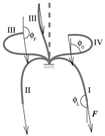
Figure 15: The shapes of an elastic beam anchored at one end and pulled by a given force $\mathbf{F}$ on its other end. The dashed line shows the unloaded beam. According to the sign of the initial curvature and the final angle $\phi_{L}$ the solutions can be divided into 4 classes. The beam corresponds to the myosin V lever arm, which is anchored in the head at one end and connected to a flexible joint at the other end. Note that the bending shown is exaggerated in comparison with realistic dimer configurations.

Because of the ambiguity of a quadratic equation, Eq. 29 generally has two solutions for a given set of values for $\phi(s)$, $F$, $\phi_{L}$ and $\phi_{F}$. As we have defined the coordinate system in a way that $\tilde{F}_{x}\geq 0$, we have $0\leq\phi_{F}\leq\pi$. We also restrict ourselves to solutions with $\left|\phi(s)\right|<2\pi$, i.e., we do not consider any spiraling solutions, because they always have a higher bending energy than the straighter solution with the same endpoint. There are four classes of functions $\phi(s)$ that satisfy the condition that the RHS of Eq. 29 be positive:

Solution	$\phi_{L}$	$\phi(s\to 0)$	conditions
I	+	+	$0\leq\phi_{L}\leq\phi_{F}$
II	-	-	$\phi_{F}-2\pi\leq\phi_{L}\leq 2\phi_{F}-2\pi$
III	+	-	$0\leq\phi_{L}\leq\phi_{F}$
IV	-	+	$\phi_{F}-2\pi\leq\phi_{L}\leq 2\phi_{F}-2\pi$

The solutions III and IV have a turning point at $\phi_{0}=-2(\pi-\phi_{F})-\phi_{L}$, where $d\phi/ds$ changes sign. Eq. 29 can finally be transformed to

$$L =\frac{1}{2}\sqrt{\frac{EI}{F}}I(\phi_{L})\qquad(\text{cases I and II})$$ (30)

$$L =\frac{1}{2}\sqrt{\frac{EI}{F}}(2I(\phi_{0})+I(\phi_{L}))\qquad(\text{cases III and IV})$$ (31)

$$I(\phi_{x}) =\left|\int_{0}^{\phi_{x}}\left(\sin\left(\frac{\phi_{L}-\phi}{2}\right)\sin\left(\phi_{F}-\frac{\phi_{L}+\phi}{2}\right)\right)^{-1/2}d\phi\right|$$

Note that for classes II and III the RHS of Eq. 30 is not monotonous in $\phi_{L}$ and there can be two solutions for a given $L$. Taking this into account, we obtain a total of up to 6 solutions. A situation in which all cases are represented is shown in Fig. 15.

The configuration of the dimer is determined by solving Eq. 15 for all possible combinations of modes and taking the one with the lowest potential. The numerical integration and solution were performed using NAG libraries (Numerical Algorithms Group) and the 3-d graphical representation of the calculated shapes was made with POV-Ray (www.povray.org).

References

- Ali et al. (2002) Ali, M. Y., S. Uemura, K. Adachi, H. Itoh, K. Kinosita Jr, and S. Ishiwata. 2002. Myosin V is a left-handed spiral motor on the right-handed actin helix. Nat. Struct. Biol. 9:464-467.
- Baker et al. (2004) Baker, J. E., E. B. Krementsova, G. G. Kennedy, A. Armstrong, K. M. Trybus, and D. M. Warshaw. 2004. Myosin V processivity: multiple kinetic pathways for head-to-head coordination. Proc. Natl. Acad. Sci. USA. 101:5542-5546.
- Burgess et al. (2002) Burgess, S., M. Walker, F. Wang, J. R. Sellers, H. D. White, P. J. Knight, and J. Trinick. 2002. The prepower stroke conformation of myosin V. J. Cell. Biol. 159:983-991.
- Clemen et al. (2003) Clemen, A., J. Jaud, M. Vilfan, and M. Rief. 2003. Private communication.
- Cooke and Pate (1985) Cooke, R., and E. Pate. 1985. The effects of ADP and phosphate on the contraction of muscle fibers. Biophys. J. 48:789-798.
- Coureux et al. (2003) Coureux, P. D., A. L. Wells, J. Menetrey, C. M. Yengo, C. A. Morris, H. L. Sweeney, and A. Houdusse. 2003. A structural state of the myosin V motor without bound nucleotide. Nature. 425:419-423.
- De La Cruz et al. (2000a) De La Cruz, E. M., H. L. Sweeney, and E. M. Ostap. 2000a. ADP inhibition of myosin V ATPase activity. Biophys. J. 79:1524-1529.
- De La Cruz et al. (1999) De La Cruz, E. M., A. L. Wells, S. S. Rosenfeld, E. M. Ostap, and H. L. Sweeney. 1999. The kinetic mechanism of myosin V. Proc. Natl. Acad. Sci. USA. 96:13726-13731.
- De La Cruz et al. (2000b) De La Cruz, E. M., A. L. Wells, H. L. Sweeney, and E. M. Ostap. 2000b. Actin and light chain isoform dependence of myosin V kinetics. Biochemistry. 39:14196-14202.
- Duke (1999) Duke, T. A. J. 1999. Molecular model of muscle contraction. Proc. Natl. Acad. Sci. USA. 96:2770-2775.
- Egelman et al. (1982) Egelman, E. H., N. Francis, and D. J. DeRosier. 1982. F-actin is a helix with a random variable twist. Nature. 298:131-135.
- Fisher and Kolomeisky (2001) Fisher, M. E., and A. B. Kolomeisky. 2001. Simple mechanochemistry describes the dynamics of kinesin molecules. Proc. Natl. Acad. Sci. USA. 98:7748-7753.
- Forkey et al. (2003) Forkey, J. N., M. E. Quinlan, M. A. Shaw, J. E. Corrie, and Y. E. Goldman. 2003. Three-dimensional structural dynamics of myosin V by single-molecule fluorescence polarization. Nature. 422:399-404.
- Hill (1974) Hill, T. L. 1974. Theoretical formalism for the sliding filament model of contraction of striated muscle. Part I. Prog. Biophys. Mol. Biol. 28:267-340.
- Howard and Spudich (1996) Howard, J., and J. A. Spudich. 1996. Is the lever arm of myosin a molecular elastic element? Proc. Natl. Acad. Sci. USA. 93:4462-4464.
- Hvidt et al. (1982) Hvidt, S., F. H. Nestler, M. L. Greaser, and J. D. Ferry. 1982. Flexibility of myosin rod determined from dilute solution viscoelastic measurements. Biochemistry. 21:4064-4073.
- Kolomeisky and Fisher (2003) Kolomeisky, A. B., and M. E. Fisher. 2003. A simple kinetic model describes the processivity of myosin-V. Biophys. J. 84:1642-1650.
- Lan and Sun (2005) Lan, G., and S. X. Sun. 2005. Dynamics of myosin-V processivity. Biophys. J. 88:999-1008.
- Lymn and Taylor (1971) Lymn, R. W., and E. W. Taylor. 1971. Mechanism of adenosine trophosphate hydrolysis by actomyosin. Biochemistry. 10:4617-4624.
- Machesky and Gould (1999) Machesky, L. M., and K. L. Gould. 1999. The Arp2/3 complex: a multifunctional actin organizer. Curr. Opin. Cell Biol. 11:117-121.
- Mehta et al. (1999) Mehta, A. D., R. S. Rock, M. Rief, J. A. Spudich, M. S. Mooseker, and R. E. Cheney. 1999. Myosin-V is a processive actin-based motor. Nature. 400:590-593.
- Molloy and Veigel (2003) Molloy, J. E., and C. Veigel. 2003. Myosin motors walk the walk. Science. 300:2045-2046.
- Moore et al. (2004) Moore, J. R., E. B. Krementsova, K. M. Trybus, and D. M. Warshaw. 2004. Does the myosin V neck region act as a lever? J. Muscle Res. Cell Motil. 25:29-35.
- Peskin et al. (1993) Peskin, C. S., G. M. Odell, and G. F. Oster. 1993. Cellular motions and thermal fluctuations: The Brownian ratchet. Biophys. J. 65:316-324.
- Peskin and Oster (1995) Peskin, C. S., and G. Oster. 1995. Coordinated hydrolysis explains the mechanical behavior of kinesin. Biophys. J. 68:202s-211s.
- Phillips and Chacko (1996) Phillips, G. N., Jr., and S. Chacko. 1996. Mechanical properties of tropomyosin and implications for muscle regulation. Biopolymers. 38:89-95.
- Purcell et al. (2002) Purcell, T. J., C. Morris, J. A. Spudich, and H. L. Sweeney. 2002. Role of the lever arm in the processive stepping of myosin V. Proc. Natl. Acad. Sci. USA. 99:14159-14164.
- Reck-Peterson et al. (2000) Reck-Peterson, S. L., D. W. Provance, Jr., M. S. Mooseker, and J. A. Mercer. 2000. Class V myosins. Biochim. Biophys. Acta. 1496:36-51.
- Rief et al. (2000) Rief, M., R. S. Rock, A. D. Mehta, M. S. Mooseker, R. E. Cheney, and J. A. Spudich. 2000. Myosin-V stepping kinetics: a molecular model for processivity. Proc. Natl. Acad. Sci. USA. 97:9482-9486.
- Rock et al. (2000) Rock, R. S., M. Rief, A. D. Mehta, and J. A. Spudich. 2000. In vitro assays of processive myosin motors. Methods. 22:373-381.
- Rosenfeld and Sweeney (2004) Rosenfeld, S. S., and H. L. Sweeney. 2004. A model of myosin V processivity. J. Biol. Chem. 279:40100-40111.
- Sakamoto et al. (2003) Sakamoto, T., F. Wang, S. Schmitz, Y. Xu, Q. Xu, J. E. Molloy, C. Veigel, and J. R. Sellers. 2003. Neck length and processivity of myosin V. J. Biol. Chem. 278:29201-29207.
- Schief and Howard (2001) Schief, W. R., and J. Howard. 2001. Conformational changes during kinesin motility. Curr. Opin. Cell Biol. 13:19-28.
- Swenson and Stellwagen (1989) Swenson, C. A., and N. C. Stellwagen. 1989. Flexibility of smooth and skeletal tropomyosins. Biopolymers. 28:955-963.
- Terrak et al. (2003) Terrak, M., G. Wu, W. F. Stafford, R. C. Lu, and R. Dominguez. 2003. Two distinct myosin light chain structures are induced by specific variations within the bound IQ motifs-functional implications. EMBO J. 22:362-371.
- Thomas et al. (2002) Thomas, N., Y. Imafuku, T. Kamiya, and K. Tawada. 2002. Kinesin: a molecular motor with a spring in its step. Proc. R. Soc. Lond. B Biol. Sci. 269:2363-2371.
- Trybus et al. (1999) Trybus, K. M., E. Krementsova, and Y. Freyzon. 1999. Kinetic characterization of a monomeric unconventional myosin V construct. J. Biol. Chem. 274:27448-27456.
- Uemura et al. (2004) Uemura, S., H. Higuchi, A. O. Olivares, E. M. De La Cruz, and S. Ishiwata. 2004. Mechanochemical coupling of two substeps in a single myosin V motor. Nat. Struct. Mol. Biol. 11:877-883.
- Vale (2003) Vale, R. D. 2003. Myosin V motor proteins: marching stepwise towards a mechanism. J. Cell. Biol. 163:445-450.
- Veigel et al. (2002) Veigel, C., F. Wang, M. L. Bartoo, J. R. Sellers, and J. E. Molloy. 2002. The gated gait of the processive molecular motor, myosin V. Nat. Cell Biol. 4:59-65.
- Vilfan and Duke (2003) Vilfan, A., and T. Duke. 2003. Instabilities in the transient response of muscle. Biophys. J. 85:818-826.
- Walker et al. (2000) Walker, M. L., S. A. Burgess, J. R. Sellers, F. Wang, J. A. Hammer, J. Trinick, and P. J. Knight. 2000. Two-headed binding of a processive myosin to F-actin. Nature. 405:804-807.
- Wang et al. (2000) Wang, F., L. Chen, O. Arcucci, E. V. Harvey, B. Bowers, Y. Xu, J. A. Hammer, and J. R. Sellers. 2000. Effect of ADP and ionic strength on the kinetic and motile properties of recombinant mouse myosin V. J. Biol. Chem. 275:4329-4335.
- Wang et al. (2003) Wang, F., K. Thirumurugan, W. F. Stafford, J. A. Hammer, P. J. Knight, and J. R. Sellers. 2003. Regulated conformation of Myosin V. J. Biol. Chem. 279:2333-2336.
- Wang et al. (1998) Wang, H. Y., T. Elston, A. Mogilner, and G. Oster. 1998. Force generation in RNA polymerase. Biophys. J. 74:1186-1202.
- Yengo et al. (2002) Yengo, C. M., E. M. De la Cruz, D. Safer, E. M. Ostap, and H. L. Sweeney. 2002. Kinetic characterization of the weak binding states of myosin V. Biochemistry. 41:8508-8517.
- Yengo and Sweeney (2004) Yengo, C. M., and H. L. Sweeney. 2004. Functional role of loop 2 in myosin V. Biochemistry. 43:2605-2612.
- Yildiz et al. (2003) Yildiz, A., J. N. Forkey, S. A. McKinney, T. Ha, Y. E. Goldman, and P. R. Selvin. 2003. Myosin V walks hand-over-hand: single fluorophore imaging with 1.5-nm localization. Science. 300:2061-2065.