Gel Electrophoresis of DNA Knots in Weak and Strong Electric Fields.

Abstract

Gel electrophoresis allows to separate knotted DNA (nicked circular) of equal length according to the knot type. At low electric fields, complex knots being more compact, drift faster than simpler knots. Recent experiments have shown that the drift velocity dependence on the knot type is inverted when changing from low to high electric fields. We present a computer simulation on a lattice of a closed, knotted, charged DNA chain drifting in an external electric field in a topologically restricted medium. Using a simple Monte Carlo algorithm, the dependence of the electrophoretic migration of the DNA molecules on the type of knot and on the electric field intensity was investigated. The results are in qualitative agreement with electrophoretic experiments done under conditions of low and high electric fields: especially the inversion of the behavior from low to high electric field could be reproduced. The knot topology imposes on the problem the constrain of self-avoidance, which is the final cause of the observed behavior in strong electric field.

Gel electrophoresis of linear and circular DNA and its dynamics has been since long time a topic on which numerical simulations and analytical models have been applied [1, 2, 3, 4, 5, 6, 7, 8].

Most experimental and theoretical studies of the electrophoresis process deal with linear or circular DNA [9, 10, 11, 12]. But DNA comes also in knotted form. Various classes of enzymes (topoisomerases and site-specific recombination enzymes) produce different types of knots or catenanes by acting on circular DNA molecules [13, 14]. The analysis of these knots gives some information about the mechanisms by which these enzymes are involved in the proper functioning of chromosomes (see for example [15]) and about DNA packing [16]. Being able to study which knots are produced by a given enzyme in prescribed conditions implies being able to perform some sort of ”knot spectroscopy”, which can be done for example by electron microscopy, where knots are observed one by one. Yet, if large numbers of knots need to be classified, then some high throughput technique is needed. Such a technique is gel electrophoresis. Indeed, experimental work has shown a linear relationship between the distance of electrophoretic migration on agarose gel of different types of DNA knots (all with the same number of base pairs) and the average crossing number of the ideal geometrical representations of the corresponding knots (closely related to the complexity of the knot)[18]. As a consequence, the type of a knot can be simply identified by measuring its position on the gel, without the need of electron microscopy experiments as required until recently.

At low electric field the usual observation is that the more complex the knot is, the higher is its mobility. A simple intuitive explanation for this behavior is that the compactness of a knot increases with its complexity (for a constant string length) and the friction coefficient $\gamma=6\pi\eta_{0}R_{H}$ (with $R_{H}$ the hydrodynamic radius of the knot and $\eta_{0}$ the viscosity of the solvent) is smaller, resulting in higher mobilities. A more refined calculation of the friction coefficient $\gamma$ relies on Kirkwood-Riseman formula [19]:

$$\gamma=\left(\sum\limits_{i=1}^{N}{\zeta_{i}}\right)\left[1+\left(6\pi\eta_{0}\sum\limits_{i=1}^{N}{\zeta_{i}}\right)^{-1}\sum\limits_{i=1}^{N}\sum\limits_{j=1}^{N}{\zeta_{i}\zeta_{j}R_{ij}^{-1}}\right]^{-1}$$ (1)

where the chain is modelled by $N$ beads of radius $\sigma_{i}$ and friction coefficent $\zeta_{i}=6\pi\eta_{o}\sigma_{i}$, and $R_{ij}$ is the distance between beads $i$ and $j$. The term $\frac{1}{R_{ij}}$, due to hydrodynamic interactions between beads, in the second factor of equation (1) explains the observed behavior: more compact molecules have smaller distances $R_{ij}$, and thus a smaller friction coefficient. The calculation of an average friction coefficient $\bar{\gamma}$ on an equilibrium set of thermally agitated DNA molecules forming different types of knots has confirmed the experimental results [20].

Recently, it was observed by two-dimensional agarose gel electrophoresis that when the strength of the electric field is increased, the electrophoretic mobility of DNA knots changes behavior (fig. 1) [17, 21]. The experiment was performed in two steps: a low strength electric field of $0.6\,Vcm^{-1}$ was first applied along one direction in the gel. At this step, more complex knots show a higher mobility, in agreement with Kirkwood-Riseman formula. The same procedure is repeated in a second step but with a stronger electric field ($5\,Vcm^{-1}$) applied perpendicularly to the first one. In this case, the opposite behavior is observed: more complex knots cover smaller distances than simple ones.

The presence of two regimes of weak and strong electric field can be captured with a simple argument. A knot of size $\xi$ drifts over a distance equal to its size along the direction of the applied electric field $\mathcal{E}$ in a time $t_{\xi}\simeq\xi/v=\gamma\xi/q\mathcal{E}$, where $v=q\mathcal{E}/\gamma$ is the drift velocity in the stationary regime and $q$ the total electrical charge carried by the DNA molecule. During the same time, the drifting knot diffuses laterally over a distance $d\simeq\sqrt{2Dt_{\xi}}=\sqrt{2\frac{k_{B}T}{\gamma}t_{\xi}}=\sqrt{2\frac{k_{B}T}{q\mathcal{E}}\xi}$, where $T$ is the absolute temperature and $k_{B}$ is the Boltzmann’s constant. If the transverse diffusion explores distances $d$ much larger than the typical size of the knot, $\xi$, then, on average, the knot will be able to avoid a collision with the gel and the knots will drift as if they were in a pure solution, with just a slight renormalization of the friction coefficient. If instead $d\ll\xi$, then whenever a knot is on a collision course with a gel strand, it can not avoid it. As a consequence, after impinging over the obstacle, the knot needs to crawl around it in order to free itself. Crawling around an obstacle is much more difficult for more complex knots than for simple ones, due to the self-avoidance constraint. Following this argument, the two electric field regimes are separated by a critical field $\mathcal{E}_{c}$ that can be obtained by setting $d\simeq\xi$, giving $\mathcal{E}_{c}\simeq 2\frac{k_{B}T}{q\xi}$. In order to estimate $\mathcal{E}_{c}$ we use the typical values for a $11^{\prime}000$ base pairs DNA knot: the size of a closed DNA ring is about $\xi=300\ nm$[22]; the total charge $q$ depends on the gel conditions, since every nucleotide carries a $P^{-}$ group, hence one electron negative charge, that can be strongly screened by charges in the solvent. As a consequence we use $q\sim 10^{-15}-10^{-16}C$. We then obtain a critical field $\mathcal{E}_{c}=0.1-1\ Vcm^{-1}$ in reasonable agreement with experiments[17, 21]. The expression for the critical electric field holds also in the case when the gel is concentrated as it is the case in many experiments. Under the condition of high gel density, the DNA is filling the pores and the expression for the collision condition is that the DNA lying between two gel strands will collide with one gel strand before the DNA can drift transversally to the electric field. Instead of $\xi$, one has to insert the gel pore size $\ell$. The lateral diffusion constant $D^{*}$ has to be rescaled in order to include the effect of the gel. The condition for the critical electric field reads again: $\mathcal{E}_{c}\simeq 2\frac{k_{B}T}{q\ell}$.

One has also to note that the two conditions for the critical electric field $\mathcal{E}_{c}$ actually mean that the energy gained by the DNA when moving one diameter $\xi$ or one pore size $\ell$ along the electric field is equal to twice the thermal energy: $q\mathcal{E}_{c}\xi$ (or $\ell$) $\simeq 2k_{B}T$. Although the above model gives a first hint of the origin of the observed behavior, here we want to address the issue more thoroughly using lattice Monte Carlo simulations.

DNA knots are modelled by closed self-avoiding walks (SAWs) composed of $N$ segments of length $a$ on a three-dimensional cubic lattice (the lattice constant $a$ is comparable to the persistence length of the DNA molecules). The gel is a two dimensional grid forming a sublattice with a mesh size $b$ (= gel parameter) and perpendicular to the applied electric field (so that no knots can ever get impaled). The gel lattice is shifted by the quantity $(\frac{a}{2},\frac{a}{2},\frac{a}{2})$ compared to the knot lattice, so that no points of the knot lie on the gel. Knots are not allowed to cross the gel network. The coordinates of the $N$ monomers in the configuration at time $t$ are written as:

$$\bar{r}(t)=(\vec{r}_{1}(t),\vec{r}_{2}(t),...,\vec{r}_{N}(t))$$ (2)

with constraints $\|\vec{r}_{j}(t)-\vec{r}_{j+1}(t)\|=a$.

The dynamics is followed using the BFACF algorithm [23]. Two types of moves are allowed: (a) the creation/destruction of a handle and (b) the flip of a corner into the mirror position (see Fig.2). The first move clearly does not preserve the knot length, which can vary by $\pm 2$ at every step, but introduces the knot elasticity. The BFACF algorithm preserves knot classes, within which it is ergodic [24]. Self-avoidance is imposed by disallowing monomers to visit any site which is already occupied by other monomers. Furthermore, knots are not allowed to cross gel rods, so that corner flips and handle creation/destruction are forbidden when a rod has to be crossed.

Under an external uniform electric field $\vec{\mathcal{E}}$, the electrostatic energy at time $t$ is given by:

$$E_{q}(t)=-\frac{q}{N(t)}\sum\limits_{j=1}^{N}{\vec{r}_{j}(t)\cdot\vec{\mathcal{E}}}.$$ (3)

$N(t)$ is the length of the knot at time $t$, and it is associated with an elastic energy

$$E_{el}(t)=\frac{1}{2}K\left[N(t)-N_{0}\right]^{2}$$ (4)

where $K$ is the spring constant. In the simulation a value $K/k_{B}T=0.1$ was used. The knot energy is then $E(t)=E_{q}(t)+E_{el}(t)$.

At each timestep, we choose a point at random on the chain and propose alternatively one of the two moves. If it satisfies the self-avoiding and gel-avoiding constraints, it is accepted with a probability given by the Metropolis algorithm: if the energy of the new trial configuration, $E_{trial}$, is lower than that of the previous configuration, $E_{old}=E(t)$, the move is accepted and $\bar{r}(t+1)=\bar{r}_{trial}$; otherwise, the probability of acceptance of the trial configuration is equal to $\exp\{-[E_{trial}-E(t)]\}/{k_{B}T}$. If the move is rejected, then $\bar{r}(t+1)=\bar{r}(t)$.

After a knotted configuration is randomly generated, the knot type is obtained by calculating its Alexander polynomial [25]. Then, we let the system freely relax to thermodynamic equilibrium in the absence of an external field ($\mathcal{E}=0$) until correlations from the initial configuration have disappeared. Then the electric field is switched on, and we let the knots migrate on the lattice. The quantities we compute are the position of the center-of-mass and the average crossing number (ACN) of the knot along a trajectory.

Time is measured in Monte Carlo iterations, length in lattice spacing. The initial length $N_{0}$ of our polymers was set to $150$, and the mean length of the knot depends generally on the electric field and on the gel parameter. However, the mean length is 145 (146) for C=0.1 (C=0.4) and b=20 and we checked that during the simulations it fluctuates around that value. The average length is slightly shorter that $N_{0}$, since the probability of shortening the polymer is a slightly larger than the probability of lengthening it due to the self-avoiding condition. The gel parameter was set to $b=5,10,20$ (in units of $a$), corresponding to a relatively sparse gel with big pores. For each initial knot, $20\cdot 10^{6}$ iterations were performed. The center-of-mass position has been measured every $1000$ Monte Carlo steps, and it was then averaged over the trajectories obtained by the migration of 100-200 different initial knots (to obtain an accuracy of about $10\%$).

One problem with the Monte Carlo algorithm is that more complex knots have a smaller drift velocity than less complex ones even in absence of the gel, when time is measured in Monte Carlo steps. This is due to the fact that already in the absence of the gel, the moves are hindered by the complexity of the knot. In order to correct this problem, we used Kirkwood-Riseman formula (1) to compute the friction coefficient $\gamma$ of every knot: since then $v=q\mathcal{E}/\gamma$, we can find the specific time rescaling necessary to go from Monte Carlo time ($t_{MC}$) to real time ($t_{R}$): $t_{R}=(\gamma v_{MC}/q\mathcal{E})t_{MC}$, where $v_{MC}$ is the velocity measured using $t_{MC}$. Once we find the time conversion (one for every knot class) in the absence of the gel, then we apply it throughout our simulations in the gel.

Let us begin with the study of the dependence of the velocity with respect to the adimensional constant $\mathcal{C}=q\mathcal{E}a/k_{B}T$ for knot type $3_{1}$ (if we assume that length fluctuations are very small, energy variations for the Metropolis algorithm can be expressed as integer multiples of $k_{B}T\mathcal{C}$). We observe two distinct behaviors for the migration of knots (see fig. 3) as a function of $\mathcal{C}$.

At high temperature or weak electric field, the distance of migration is linear as a function of $\mathcal{C}$. On the other hand, above a critical value of $\mathcal{C}_{crit}$, the average speed of the knots is decreasing with $\mathcal{C}$, in qualitative agreement with the experimental results. For our parameters, $\mathcal{C}_{crit}$ is located around $0.4$ for the $3_{1}$ knot. Clearly, this value depends on the length of the knot and on its type (it can also depend on the gel parameter $b$ if $b<\xi$, the typical size of the knot). If the electric field is strong, or temperature is low, knots tend to hang over obstacles and take a U-shape configuration. When a knot hits a gel rod, it can easily remain trapped there, because the probability of a backward step is very small, and it is a growing function of the temperature $T$. Trapping in U-shape conformations introduces plateaus in the migration distance as a function of time for individual knots, hence reducing the average migration velocity. On the same graph (fig. 3), the drift velocity for a $8_{1}$ knot is depicted as a function of $\mathcal{C}$. The general behavior is similar to the $3_{1}$ knot, but the drift speed at low $\mathcal{C}$ is higher than for the $3_{1}$ knot (as it is the case in the experiments). But the most striking feature is that at $\mathcal{C}\approx 0.2-0.3$ the two curves cross each other and the $3_{1}$ is faster than the $8_{1}$ for $\mathcal{C}>0.3$. This is also the observed behavior in the experiments.

We investigate now the effect of the knot type for both weak and strong electric fields ($\mathcal{C}=0.1$ and $\mathcal{C}=0.4$ respectively) for eleven types of knots ($3_{1}$, $4_{1}$, $5_{1}$, $5_{2}$, $6_{1}$, $6_{2}$, $6_{3}$, $7_{1}$, $7_{2}$, $7_{3}$ and $8_{1}$) all consisting of 150 monomers. For each knot type, we extract the average velocity from the distance of migration vs. time curve. The velocity of migration is then plotted as a function of the measured ACN, that is related to the knot type. This plot is done first only for the high electric field case ($\mathcal{C}=0.4$) in fig. 4. We observe that there is a fairly linear relationship (except for the $3_{1}$ knot) between the average velocity of knots and the ACN (measure of complexity). More complex knots migrate slower than simpler ones at strong electric fields (although much noisier than for weak fields). These results are in agreement with experiments. A similar plot was done for the low electric field ($\mathcal{C}=0.1$) and the results are depicted in fig. 5 (filled squares).

The intuitive view of a knot making its way through the pores of the gel would have as a consequence that more complex (thus more compact) knots migrate faster than simple knots, because they are less disturbed by the gel. This is indeed what happens in weak electric fields. In the strong field regime our simulations are in agreement with experiments and show the opposite behavior, indicating that the knot collides with the gel and that the condition of self-avoidance makes the migration of compact knots around the gel strands more difficult. Somehow, parts of the knot have to go around other parts of itself, a process which is much longer for complex knots than for simple knots.

The trapping of linear open polymers in U-shape conformations is actually an artifact: indeed the slightest difference in the length of the two arms of the U gives rise to a net electric force that allows the polymer to slide around the obstacle. Simple local Monte Carlo moves do not allow to capture this dynamics. Yet, adding suitable non-local moves is enough to eliminate the artificious slowing down of the dynamics and cures the exponentially long relaxation times of thermal activation around the obstacle [6, 28]. However, the closed knot topology of DNA in our numerical simulations does not allow to introduce the long range moves. Moreover, we argue that exponentially long relaxation times present in our simulations affect, in first approximation, all the knots irrespective of their topology. In the ideal case of purely mechanical and frictionless unbinding, one can easily check that the knot complexity introduces at most a small logarithmic correction according to which more complex knots would anyway unpin faster in contradiction with both experiments and our simulation. Therefore, the simulated absolute drift velocity $v_{abs}$ is affected by a time scale that is artificially stretched in essentially the same way independent on the knot class. So, by looking at the ratios of the absolute velocities, this time scale should in first approximation cancel out. In Figure 5 we plot the simulated and experimental ratios $v_{m.n}^{abs}/v_{3.1}^{abs}$ as function of the ACN. In this Figure the open points represent data from Sogo et al.[21], and the filled symbols our simulation results. The ACN values for each knot were taken from Vologdskii et al. [20]. The agreement between experimental data and simulations is remarkable. In weak electric field, the transport properties of DNA knots are dominated by the hydrodynamics of the knots and the gel plays a minor role. At high electric fields, the knot-gel interaction is predominant and it is responsible for the inversion of behavior. In particular, strong DNA-gel interactions enhance the effect of self-avoidance within the knotted DNA and self-avoidance must be included in simulations in order to reproduce the correct behavior. This is at variance with simulations of gel electrophoresis of linear DNA where self-avoidance is usually neglected because of the two following reasons: first, according to the repton model, DNA crawls along tubes in the gel and it is in an elongated configuration where self-intersections are negligible. Secondly, it is often assumed that the drifting DNA can be considered to be in a semi-dilute solution regime, where polymers obey random walk statistics. Instead, in our case the conservation of the knot topology during the dynamics imposes the inclusion of self-avoidance.

We presented some results of a Monte Carlo simulation of DNA knots in a gel in three dimensions. In summary, our model allows to explain the high electric field behavior observed in experimental DNA knots gel electrophoresis. The variation of the gel parameter does not change qualitatively the results. However, in a denser gel, the knots get stuck at shorter distances. In a more realistic modelization of the gel, the gel fibers should be allowed to break and let the knots migrate further. Varying the length of the knots would probably also bring some further insights into the mechanisms of the migration in a gel.

We thank X. Zotos, A. Baldereschi, A. Stasiak, J. Roca, J. Schvartzman, and G. D’Anna for help and for fruitful discussions. This work was partially supported by the Swiss National Science Foundation (Grant Nr. 21-50805.97)

Figure Captions

• Figure 1: Analysis by two-dimensional agarose gel electrophoresis of pH5.8 DNA (8749 bp) with the diagrammatic interpretation of the autoradiogram and the standard agarose electrophoresis (left panel). Reproduced from [21] with permission.

• Figure 2: Elementary moves of the BFACF algorithm. a) creation of a handle (the opposite move destroys a handle) and b) corner flip.

• Figure 3: Drift velocity in arbitrary units for the $3_{1}$ (open circles) and $8_{1}$ (filled circles) knots as function of $\mathcal{C}=q\mathcal{E}a/k_{B}T$. The lines are only guides for the eyes.

• Figure 4: Linear relation between the electrophoretic drift velocity of the centre-of-mass as a function of the average crossing number (determined during the simulation) for different knots for low and high electric field (filled circles for $\mathcal{C}=0.1$, open circles for $\mathcal{C}=0.4$).

• Figure 5: Distance of migration in gel for the experimental data or drift velocity for the simulated data vs. ACN (from [20]) for knots from $3_{1}$ to $8_{1}$. Open symbols are data from Sogo et al. [21], filled symbols are the simulated values of the drift velocity. Squares are for low electric field ($\mathcal{E}=0.6\ V/cm$ and $\mathcal{C}=0.1$, respectively), while triangles are for high electric field ($\mathcal{E}=5\ V/cm$ and $\mathcal{C}=0.4$). The values were all normalized to their respective value for the knot $3_{1}$.

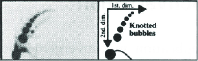
Figure 1: Analysis by two-dimensional agarose gel electrophoresis of pH5.8 DNA (8749 bp) with the diagrammatic interpretation of the autoradiogram and the standard agarose electrophoresis (left panel). Reproduced from [21] with permission.

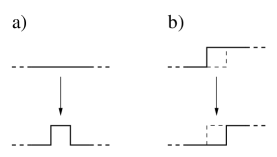
Figure 2: Elementary moves of the BFACF algorithm. a) creation of a handle (the opposite move destroys a handle) and b) corner flip.

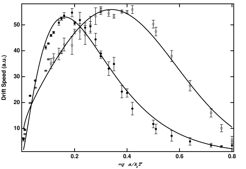
Figure 3: Drift velocity in arbitrary units for the $3_{1}$ (open circles) and $8_{1}$ (filled circles) knots as function of $\mathcal{C}=q\mathcal{E}a/k_{B}T$. The lines are only guides for the eyes.

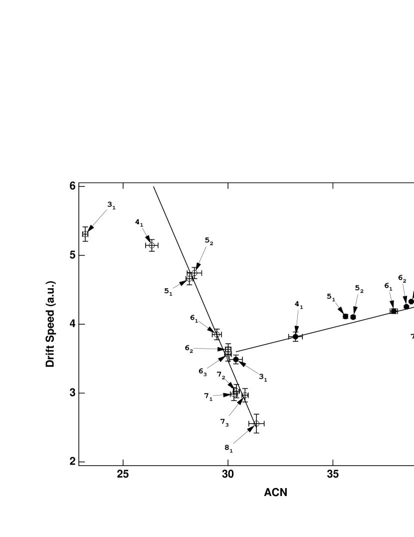
Figure 4: Linear relation between the electrophoretic drift velocity of the centre-of-mass as a function of the average crossing number (determined during the simulation) for different knots for low and high electric field (filled circles for $\mathcal{C}=0.1$, open circles for $\mathcal{C}=0.4$).

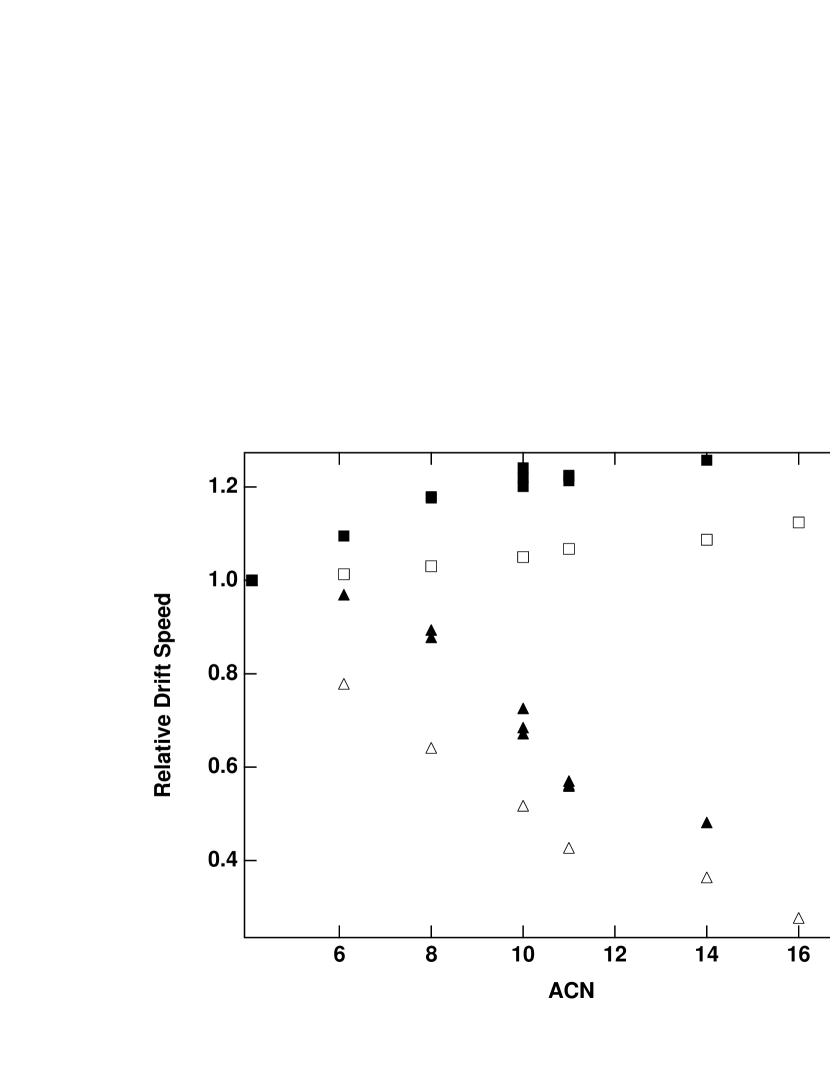
Figure 5: Distance of migration in gel for the experimental data or drift velocity for the simulated data vs. ACN (from [20]) for knots from $3_{1}$ to $8_{1}$. Open symbols are data from Sogo et al. [21], filled symbols are the simulated values of the drift velocity. Squares are for low electric field ($\mathcal{E}=0.6\ V/cm$ and $\mathcal{C}=0.1$, respectively), while triangles are for high electric field ($\mathcal{E}=5\ V/cm$ and $\mathcal{C}=0.4$). The values were all normalized to their respective value for the knot $3_{1}$.

References

- [*] Corresponding author: Giovanni Dietler, Laboratoire de Physique de la Matière Vivante, Faculté des Sciences de Base, Ecole Polytechnique Fédérale de Lausanne, CH-1015 Lausanne. Tel: (+41) 21 693 0446, FAX (+41) 21 693 0422, email: giovanni.dietler@epfl.ch
- [1] Noolandi, J., Rousseau, J., Slater, G.W., Turmel, C., & Lalande, M., (1987) Phys. Rev. Lett. 58, 2428-2431.
- [2] Deutsch, J.M., (1988) Science 240, 922-924 .
- [3] Viovy, J.L., (1988) Phys. Rev. Lett. 60, 855-858.
- [4] Doi, M., Kobayashi, T., Makino, Y., Ogawa, M., Slater , G.W., & Noolandi, J., (1988) Phys. Rev. Lett. 61, 1893-1896.
- [5] Noolandi, J., Slater, G.W., Lim, H.A., & Joanny, J.-F., (1989) Science 243, 1456-1458.
- [6] Duke , T.A.J. & Viovy, J.L., (1992) Phys. Rev. Lett. 68, 542-545.
- [7] Aalberts, D.P., (1995) Phys. Rev. Lett. 75, 4544-4547.
- [8] Semenov, A.N. & Joanny, J.-F., (1997) Phys Rev. E 55, 789-799.
- [9] Schwartz, D.C. & Koval, M., (1989) Nature 338, 520-522.
- [10] Smith, S.B., Aldridge, P.K., & Callis, J.B., (1989) Science 243, 203-206.
- [11] Sturm, J. & Weill, G., (1989) Phys. Rev. Lett. 62, 1484-1487.
- [12] Wang Z.L., & Chu, B., (1989) Phys. Rev. Lett. 63, 2528-2531.
- [13] Dean, F.B., Stasiak, A., Koller, T., & Cozzarelli, N.R., (1985) J. Biol. Chem. 260, 4975-4983.
- [14] Spengler, S.J., Stasiak, A., & Cozzarelli, N.R., (1985) Cell 42, 325-334.
- [15] Duplantier, B., Jannink, G., & Sikorav, J.L., (1995) Biophys. J. 69, 1596-1605.
- [16] Arsuaga, J., Vazquez, M., Trigueros, S., Sumners, D., & Roca, J., (2002) PNAS 99, 5373-5377.
- [17] Trigueros, S., Arsuaga, J., Vazquez, M.E., Sumners, D.W., & Roca, J., (2001) Nucl. Acid. Res. 29, e67.
- [18] Stasiak, A., Katritch, V., Bednar, J., Michoud, M., & Dubochet, J., (1996) Nature 384, 122-122.
- [19] De la Torre, J.G., & Bloomfield, V.A., (1981) Quarterly Reviews of Biophysics 14, 81-139.
- [20] Vologodskii, A.V., Crisona, N.J., Laurie, B., Pieranski, P., Katritch, V., Dubochet, J., & Stasiak, A., (1998) J. Mol. Biol. 278, 1-3.
- [21] Sogo, J., Stasiak, A., Martinez-Robles, M.L., Krimer, D.B., Hernandez, P., & Schvartzman, J.B., (1999) J. Mol. Biol. 286, 637-643.
- [22] This value is estimated from Atomic Force Images of complex knots. The knots were kindly provided by Dr. J. Roca and the AFM images were taken by Dr. F. Valle.
- [23] Berg, B., & Foerster, D., (1981) Phys. Lett. B 106, 323-326; Aragão de Carvalho, C., Caracciolo, S., & Fröhlich, J., (1983) Nucl. Phys. B 215, 209-248; see also Lim, H.A., (1996) Intl. J. Mod. Phys. C 7, 217-271 and references therein.
- [24] van Rensburg, E.J.J., & Whittington, S.G., (1991) J. Phys. A 24, 5553-5567.
- [25] Alexander, J.W., (1923) Trans. Amer. Math. Soc. 20, 275-306.
- [26] Grosberg, A.Y., (2000) Phys. Rev. Lett. 85, 3858-3861.
- [27] Dobay, A., Dubochet, J., Millett, K., Sottas, P.E., & Stasiak, A., (2003) PNAS 100, 5611-5615.
- [28] van Heukelum, A., & Barkema, G.T., (2002) Electrophoresis 23, 2562-2568.