Orientational instabilities in nematics with weak anchoring
under combined action of steady flow and external fields

Abstract

We study the homogeneous and the spatially periodic instabilities in a nematic liquid crystal layer subjected to steady plane Couette or Poiseuille flow. The initial director orientation is perpendicular to the flow plane. Weak anchoring at the confining plates and the influence of the external electric and/or magnetic field are taken into account. Approximate expressions for the critical shear rate are presented and compared with semi-analytical solutions in case of Couette flow and numerical solutions of the full set of nematodynamic equations for Poiseuille flow. In particular the dependence of the type of instability and the threshold on the azimuthal and the polar anchoring strength and external fields is analysed.

I Introduction

Nematic liquid crystals (nematics) represent the simplest anisotropic fluid. The description of the dynamic behavior of the nematics is based on well established equations. The description is valid for low molecular weight materials as well as nematic polymers.

The coupling between the preferred molecular orientation (director $\boldsymbol{\rm\hat{n}}$) and the velocity field leads to interesting flow phenomena. The orientational dynamics of nematics in flow strongly depends on the sign of the ratio of the Leslie viscosity coefficients $\lambda=\alpha_{3}/\alpha_{2}$.

In typical low molecular weight nematics $\lambda$ is positive (flow-aligning materials). The case of the initial director orientation perpendicular to the flow plane has been clarified in classical experiments by Pieranski and Guyon Pieranski and Guyon (1973, 1974) and theoretical works of Dubois-Violette and Manneville (for an overview see Dubois-Violette and Manneville (1996)). An additional external magnetic field could be applied along the initial director orientation. In Couette flow and low magnetic field there is a homogeneous instability Pieranski and Guyon (1973). For high magnetic field the homogeneous instability is replaced by a spatially periodic one leading to rolls Pieranski and Guyon (1974). In Poiseuille flow, as in Couette flow, the homogeneous instability is replaced by a spatially periodic one with increasing magnetic field Manneville (1979). All these instabilities are stationary.

Some nematics (in particular near a nematic-smectic transition) have negative $\lambda$ (non-flow-aligning materials). For these materials in steady flow and in the geometry where the initial director orientation is perpendicular to the flow plane only spatially periodic instabilities are expected Pieranski and Guyon (1976). These materials demonstrate also tumbling motion Cladis and Torza (1975) in the geometry where the initial director orientation is perpendicular to the confined plates that make the orientational behavior quite complicated.

Most previous theoretical investigations of the orientational dynamics of nematics in shear flow were carried out under the assumption of strong anchoring of the nematic molecules at the confining plates. However, it is known that there is substantial influence of the boundary conditions on the dynamical properties of nematics in hydrodynamic flow Kedney and Leslie (1998); Nasibullayev et al. (2000); Tarasov et al. (2001); Nasibullayev and Krekhov (2001). Indeed, the anchoring strength strongly influences the orientational behavior and dynamic response of nematics under external electric and magnetic fields. This changes, for example, the switching times in bistable nematic cells Kedney and Leslie (1998), which play an important role in applications Chigrinov (1999). Recently the influence of the boundary anchoring on the homogeneous instabilities in steady flow was investigated theoretically Tarasov et al. (2001).

In this paper we study the combined action of steady flow (Couette and Poiseuille) and external fields (electric and magnetic) on the orientational instabilities of the nematics with initial orientation perpendicular to the flow plane. We focus on flow-aligning nematics. The external electric field is applied across the nematic layer and the external magnetic field is applied perpendicular to the flow plane. We analyse the influence of weak azimuthal and polar anchoring and of external fields on both homogeneous and spatially periodic instabilities.

In section II the formulation of the problem based on the standard set of Ericksen-Leslie hydrodynamic equations Leslie (1976) is presented. Boundary conditions and the critical Freédericksz field in case of weak anchoring are discussed. In section III equations for the homogeneous instabilities are presented. Rigorous semi-analytical expressions for the critical shear rate $a_{c}^{2}$ for Couette flow (section III A), the numerical scheme for finding $a_{c}^{2}$ for Poiseuille flow (section III B) and approximate analytical expressions for both types of flows (section III C) are presented. In section IV the analysis of the spatially periodic instabilities is given and in section V we discuss the results. In particular we will be interested in the boundaries in parameter space (anchoring strengths, external fields) for the occurrence of the different types of instabilities.

II Basic equations

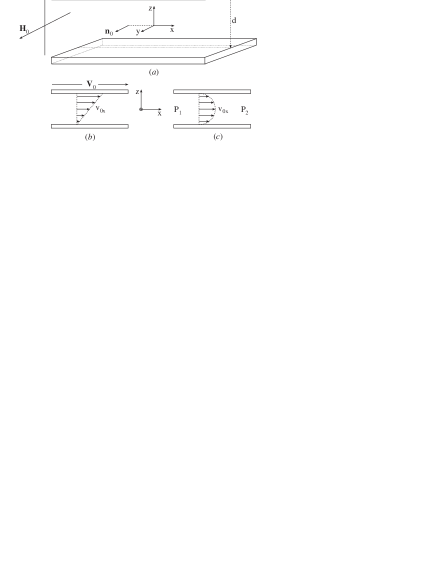
Figure 1: Geometry of NLC cell ($a$). Couette ($b$) and Poiseuille ($c$) flows.

Consider a nematic layer of thickness $d$ sandwiched between two infinite parallel plates that provide weak anchoring (Fig. 1 $a$). The origin of the Cartesian coordinates is placed in the middle of the layer with the $z$ axis perpendicular to the confining plates ($z=\pm d/2$ for the upper/lower plate). The flow is applied along $x$. Steady Couette flow is induced by moving the upper plate with a constant speed (Fig. 1 $b$). Steady Poiseuille flow is induced by applying a constant pressure difference along $x$ (Fig. 1 $c$). An external electric field $E_{0}$ is applied along $z$ and a magnetic field $H_{0}$ along $y$.

The nematodynamic equations have the following form de Gennes (1974)

$$\rho(\partial_{t}+\boldsymbol{\rm v}\cdot\boldsymbol{\rm\nabla})v_{i}=-p_{,i}+[T^{v}_{ji}+T^{e}_{ji}]_{,j},$$ (1)

$$\gamma_{1}\boldsymbol{\rm N}=-(1-\boldsymbol{\rm n}\boldsymbol{\rm n}\cdot)(\gamma_{2}A\cdot\boldsymbol{\rm n}+\boldsymbol{\rm h}),$$ (2)

where $\rho$ is the density of the NLC and $p_{,i}=\Delta P/\Delta x$ the pressure gradient; $\gamma_{1}=\alpha_{3}-\alpha_{2}$ and $\gamma_{2}=\alpha_{3}+\alpha_{2}$ are rotational viscosities; $\boldsymbol{\rm N}=\boldsymbol{\rm n}_{,t}+\boldsymbol{\rm v}\cdot\boldsymbol{\rm\nabla}\boldsymbol{\rm n}-(\nabla\times\boldsymbol{\rm v})\times\boldsymbol{\rm n}/2$ and $A_{ij}=(v_{i,j}+v_{j,i})/2$, $h_{i}=\delta F/\delta n_{i}$. The notation $f_{,i}\equiv\partial_{i}f$ is used throughout. The viscous tensor $T^{v}_{ij}$ and elastic tensor $T^{e}_{ij}$ are

$$T^{v}_{ij}= \alpha_{1}n_{i}n_{j}A_{km}n_{k}n_{m}+\alpha_{2}n_{i}N_{j}+\alpha_{3}n_{j}N_{i}$$ (3)

$$+\alpha_{4}A_{ij}+\alpha_{5}n_{i}n_{k}A_{ki}+\alpha_{6}A_{ik}n_{k}n_{j},$$

$$T^{e}_{ij}= -\frac{\partial F}{\partial n_{k,i}}n_{k,j},$$ (4)

where $\alpha_{i}$ are the Leslie viscosity coefficients. The bulk free energy density $F$ is

$$F= \frac{1}{2}\Bigl{\{}K_{11}(\nabla\cdot\boldsymbol{\rm n})^{2}+K_{22}[\boldsymbol{\rm n}\cdot(\nabla\times\boldsymbol{\rm n})]^{2}$$

$$+K_{33}[\boldsymbol{\rm n}\times(\nabla\times\boldsymbol{\rm n})]^{2}-\varepsilon_{0}\varepsilon_{a}(\boldsymbol{\rm n}\cdot\boldsymbol{\rm E}_{0})^{2}$$

$$-\mu_{0}\chi_{a}(\boldsymbol{\rm n}\cdot\boldsymbol{\rm H}_{0})^{2}\Bigr{\}}.$$

Here $K_{ii}$ are the elastic constants, $\varepsilon_{a}$ the anisotropy of the dielectric permittivity and $\chi_{a}$ is the anisotropy of the magnetic susceptibility.

In addition one has the normalization equation

$$\boldsymbol{\rm n}=1$$ (6)

and incompressibility condition

$$\nabla\cdot\boldsymbol{\rm v}=0.$$ (7)

The basic state solution of equations (1) and (2) has the following form

$$\boldsymbol{\rm n}_{0}=(0,\>1,\>0),\>\boldsymbol{\rm v}_{0}=(v_{0x}(z),\>0,\>0),$$ (8)

where $v_{0x}=V_{0}(1/2+z/d)$ for Couette and $v_{0x}=(\Delta P/\Delta x)[d^{2}/\alpha_{4}][1/4-z^{2}/d^{2}]$ for Poiseuille flow.

In order to investigate the stability of the basic state (8) with respect to small perturbations we write:

$$\boldsymbol{\rm n}=\boldsymbol{\rm n}_{0}+\boldsymbol{\rm n}_{1}(z)e^{\sigma t}e^{iqy},\>\boldsymbol{\rm v}=\boldsymbol{\rm v}_{0}+\boldsymbol{\rm v}_{1}(z)e^{\sigma t}e^{iqy};$$ (9)

We do not expect spatial variation along $x$ for steady flow. The case $q=0$ corresponds to a homogeneous instability. Here we analyse stationary bifurcations, thus the threshold condition is $\sigma=0$.

Introducing the dimensionless quantities in terms of layer thickness $d$ (typical length) and director relaxation time $\tau_{d}=(-\alpha_{2})d^{2}/K_{22}$ (typical time) the linearised equations (1) and (2) can be rewritten in the form

$$(\eta_{13}-1)q^{2}Sn_{1z}+iq(\eta_{13}q^{2}-\partial_{z}^{2})v_{1x}=0,$$ (10a)

$$\partial_{z}[\eta_{52}q^{2}+(1-\eta_{32})\partial_{z}^{2}](Sn_{1x})$$

$$\quad+(\eta_{12}q^{4}-\eta_{42}q^{2}\partial_{z}^{2}+\partial_{z}^{4})v_{1y}=0,$$ (10b)

$$(\partial_{z}^{2}-k_{32}q^{2}-h)n_{1x}+Sn_{1z}+iqv_{1x}=0,$$ (10c)

$$\partial_{z}(k_{12}\partial_{z}^{2}-k_{32}q^{2}-h+k_{12}e)n_{1z}$$

$$\quad+\lambda\partial_{z}(Sn_{1x})-(q^{2}+\lambda\partial_{z}^{2})v_{1y}=0,$$ (10d)

$$v_{1z,z}=-iqv_{1y}.$$ (10e)

where $\eta_{ij}=\eta_{i}/\eta_{j}$, $\eta_{1}=(\alpha_{4}+\alpha_{5}-\alpha_{2})/2$, $\eta_{2}=(\alpha_{3}+\alpha_{4}+\alpha_{6})/2$, $\eta_{3}=\alpha_{4}/2$, $\eta_{4}=\alpha_{1}+\eta_{1}+\eta_{2}$, $\eta_{5}=-(\alpha_{2}+\alpha_{5})/2$, $k_{ij}=K_{ii}/K_{jj}$, $\lambda=\alpha_{3}/\alpha_{2}$, $h=\pi^{2}H_{0}^{2}/H_{F}^{2}$, $e=\operatorname{sgn}(\varepsilon_{a})\pi^{2}E_{0}^{2}/E_{F}^{2}$ and $H_{F}=(\pi/d)\sqrt{K_{22}/(\mu_{0}\chi_{a})}$, $E_{F}=(\pi/d)\sqrt{K_{11}/(\varepsilon_{0}|\varepsilon_{a}|)}$ are the critical Fréedericksz transition fields for strong anchoring.

For the shear rate $S$ one has, for Couette flow,

$$S=a^{2},\>a^{2}=\dfrac{V_{0}\tau_{d}}{d}$$ (11)

and for Poiseuille flow

$$S=-a^{2}z,\>a^{2}=-\dfrac{\Delta P}{\Delta x}\dfrac{\tau_{d}d}{\eta_{3}}.$$ (12)

The anchoring properties are characterised by a surface energy per unit area, $F_{s}$, which has a minimum when the director at the surface is oriented along the easy axis (parallel to the $y$ axis in our case). A phenomenological expression for the surface energy $F_{s}$ can be written in terms of an expansion with respect to $(\boldsymbol{\rm n}-\boldsymbol{\rm n}_{0})$. For small director deviations from the easy axis one obtains

$$F_{s}=\frac{1}{2}W_{a}n_{1x}^{2}+\frac{1}{2}W_{p}n_{1z}^{2},\quad W_{a}>0,\>W_{p}>0,$$ (13)

where $W_{a}$ and $W_{p}$ are the “azimuthal” and “polar” anchoring strengths, respectively. $W_{a}$ characterizes the surface energy increase due to distortions within the surface plate and $W_{p}$ relates to distortions out of the substrate plane.

The boundary conditions for the director perturbations can be obtained from the torques balance equation

$$\pm\frac{\partial F}{\partial(\partial n_{1i}/\partial z)}+\frac{\partial F_{s}}{\partial n_{1i}}=0,$$ (14)

with “$\pm$” for $z=\pm d/2$. The boundary conditions (13) can be rewritten in dimensionless form as:

$$\pm\beta_{a}n_{1x,z}+n_{1x}=0,\>\pm\beta_{p}n_{1z,z}+n_{1z}=0,$$ (15)

with “$\pm$” for $z=\pm 1/2$. Here we introduced dimensionless anchoring strengths as ratios of the characteristic anchoring length ($K_{ii}/W_{i}$) over the layer thickness $d$:

$$\beta_{a}=K_{22}/(W_{a}d),\>\beta_{p}=K_{11}/(W_{p}d).$$ (16)

In the limit of strong anchoring, $(\beta_{a},\>\beta_{p})\to 0$, one has $n_{1x}=n_{1z}=0$ at $z=\pm 1/2$. For torque-free boundary conditions, $(\beta_{a},\>\beta_{p})\to\infty$, one has $n_{1x,z}=n_{1z,z}=0$ at the boundaries. From (16) one can see that by changing the thickness $d$, the dimensionless anchoring strengths $\beta_{a}$ and $\beta_{p}$ can be varied with the ratio $\beta_{a}/\beta_{p}$ remaining constant.

The boundary conditions for the velocity field (no-slip) are

$$v_{1x}(z=\pm 1/2)=0;$$ (17)

$$v_{1y}(z=\pm 1/2)=0;$$ (18)

$$v_{1z}(z=\pm 1/2)=v_{1z,z}(z=\pm 1/2)=0.$$ (19)

The existence of a nontrivial solution of the linear ordinary differential equations (10) with the boundary conditions (15), (17 – 19) gives values for the shear rate $S_{0}(q)$ (neutral curve). The critical value $S_{c}(q_{c})$, above which the basic state (8) becomes unstable, are given by the minimum of $S_{0}$ with respect to $q$.

Table 1: Symmetry properties of the solutions of equations (10) under $\{z\to-z\}$.

	Couette flow		Poiseuille flow
Perturbation	“odd”	“even”	“odd”	“even”
$n_{1x}$	odd	even	odd	even
$n_{1z}$	odd	even	even	odd
$v_{1x}$	odd	even	odd	even
$v_{1y}$	even	odd	odd	even
$v_{1z}$	odd	even	even	odd

The symmetry properties of the solutions of equations (10) under the reflection $z\to-z$ is shown in the Table 1. We will always classify the solutions by the $z$ symmetry of the $x$ component of the director perturbation $n_{1x}$ (first row in Table I).

In case of positive $\varepsilon_{a}$, for some critical value of the electric field the basic state loses its stability already in the absence of flow (Freédericksz transition). Clearly the Freédericksz transition field depends on the polar anchoring strength. There is competition of the elastic torque $K_{11}n_{1z,zz}$ and the field-induced torque $\varepsilon_{a}\varepsilon_{0}E_{0}^{2}n_{1z}$. The solution of Eq. (10) with $n_{1x}=0$, $v_{1y}=0$ for $h=0$ has the form

$$n_{1z}=C\cos(\pi\delta z/d),$$ (20)

where $\delta=E_{F}^{weak}/E_{F}$ and $E_{F}^{weak}$ is the actual Fréedericksz field.

After substituting $n_{1z}$ into the boundary conditions (15) we obtain the expression for $\delta$:

$$\tan\dfrac{\pi\delta}{2}=\dfrac{1}{\pi\beta_{p}\delta}.$$ (21)

One easily sees that $\delta\to 1$ for $\beta_{p}\to 0$ and $\delta\to\sqrt{2/\beta_{p}}/\pi$ for $\beta_{p}\to\infty$. For $\beta_{p}=1$ one gets $E_{F}^{weak}=0.42E_{F}$.

III Homogeneous instability

In order to obtain simpler equations we use the renormalized variables as in Ref. Tarasov et al. (2001):

$$\tilde{S}=\beta^{-1}S,\>N_{1x}=\beta^{-1}n_{1x},\>N_{1z}=n_{1z},\>V_{1x}=\beta^{-1}v_{1x},$$

$$V_{1y}=(\beta^{2}\eta_{23})^{-1}v_{1y},\>V_{1z}=(\beta^{2}\eta_{23})^{-1}v_{1z}$$ (22)

with

$$\beta^{2}=\alpha_{32}k_{21}\eta_{32},\>\alpha_{ij}=\dfrac{\alpha_{i}}{\alpha_{j}}.$$ (23)

In the case of homogeneous perturbations ($q=0$) Eqs. (10) reduce to $V_{1z}=0$ and

$$V_{1y,zz}-(1-\eta_{23})(\tilde{S}N_{1x})_{,z}=0,$$ (24a)

$$\tilde{S}N_{1z}-N_{1x,zz}+hN_{1x}=0,$$ (24b)

$$\eta_{23}\tilde{S}N_{1x}+N_{1z,zz}-V_{1y,z}-(k_{21}h-e)N_{1z}=0.$$ (24c)

III.1 Couette flow

For Couette flow we can obtain the solution of (24) semi-analytically. For the “odd” solution one gets

$$N_{1x}=C_{1}\sinh(\xi_{1}z)+C_{2}\sin(\xi_{2}z),$$ (25)

$$N_{1z}=C_{3}\sinh(\xi_{1}z)+C_{4}\sin(\xi_{2}z),$$ (26)

$$V_{1y}=C_{5}\cosh(\xi_{1}z)+C_{6}\cos(\xi_{2}z)+C_{7}.$$ (27)

Taking into account the boundary conditions (15, 18) the solvability condition for the $C_{i}$ (“boundary determinant” equal to zero) gives an expression for the critical shear rate $a_{c}$:

$$(h+\xi_{2}^{2})[\xi_{1}\beta_{a}\cosh(\xi_{1}/2)+\sinh(\xi_{1}/2)]\\ \times[\xi_{2}\beta_{p}\cos(\xi_{2}/2)+\sin(\xi_{2}/2)]\\ -(h-\xi_{1}^{2})[\xi_{2}\beta_{a}\cos(\xi_{2}/2)+\sin(\xi_{2}/2)]\\ \times[\xi_{1}\beta_{p}\cosh(\xi_{1}/2)+\sinh(\xi_{1}/2)]=0.$$ (28)

where

$$\xi_{1}^{2}=\dfrac{[(1+k_{12})h-k_{12}e]+\xi}{2k_{12}},$$ (29)

$$\xi_{2}^{2}=\dfrac{-[(1+k_{12})h-k_{12}e]+\xi}{2k_{12}},$$ (30)

$$\xi=\sqrt{[(1-k_{12})h-k_{12}e]^{2}+4k_{12}^{2}a^{4}}.$$ (31)

For the “even” solution one obtains:

$$N_{1x}=C_{1}\cosh(\xi_{1}z)+C_{2}\cos(\xi_{2}z)+C_{3},$$ (32)

$$N_{1z}=C_{4}\cosh(\xi_{1}z)+C_{5}\cos(\xi_{2}z)+C_{6},$$ (33)

$$V_{1y}=C_{7}\sinh(\xi_{1}z)+C_{8}z.$$ (34)

The boundary conditions (17-19) now lead to the following condition (“boundary determinant”):

$$\begin{vmatrix}1&h&\dfrac{\eta_{23}}{2}\left(\dfrac{h(h-k_{12}e)}{a^{4}k_{12}\eta_{23}}-1\right)\\ -\xi_{2}\beta_{a}\sin(\xi_{2}/2)+\cos(\xi_{2}/2)&(h+\xi_{2}^{2})[-\xi_{2}\beta_{p}\sin(\xi_{2}/2)+\cos(\xi_{2}/2)]&\dfrac{1-\eta_{23}}{\xi_{2}}\sin(\xi_{2}/2)\\ \xi_{1}\beta_{a}\sinh(\xi_{1}/2)+\cosh(\xi_{1}/2)&(h-\xi_{1}^{2})[\xi_{1}\beta_{p}\sinh(\xi_{1}/2)+\cosh(\xi_{1}/2)]&\dfrac{1-\eta_{23}}{\xi_{1}}\sinh(\xi_{1}/2)\end{vmatrix}=0.$$ (35)

III.2 Poiseuille flow

In the case of Poiseuille flow the system (24) with $\tilde{S}=-za^{2}/\beta$ admits an analytical solution only in the absence of external fields (in terms of Airy functions) Tarasov et al. (2001). In the presence of fields we solve the problem numerically. In the framework of the Galerkin method we expand $N_{1x}$, $N_{1z}$ and $V_{1y}$ in a series

$$N_{1x}=\sum\limits_{n=1}^{\infty}C_{1,n}f_{n}(z),$$

$$N_{1z}=\sum\limits_{n=1}^{\infty}C_{2,n}g_{n}(z),$$ (36)

$$V_{1y}=\sum\limits_{n=1}^{\infty}C_{3,n}u_{n}(z),$$

where the trial functions $f_{n}$, $g_{n}$ and $u_{n}$ satisfy the boundary conditions (15), (18). For the “odd” solution we write

$$f_{n}(z)=\zeta_{n}^{o}(z;\beta_{a}),\;g_{n}(z)=\zeta_{n}^{e}(z;\beta_{p}),\>u_{n}(z)=\nu_{n}^{o}(z)$$ (37)

and for the “even” solution

$$f_{n}(z)=\zeta_{n}^{e}(z;\beta_{a}),\;g_{n}(z)=\zeta_{n}^{o}(z;\beta_{p}),\>u_{n}(z)=\nu_{n}^{e}(z).$$ (38)

The functions $\zeta_{n}^{o}(z;\beta)$, $\zeta_{n}^{e}(z;\beta)$, $\nu_{n}^{o}(z)$, $\nu_{n}^{e}(z)$ are given in Appendix A. In our calculations we have to truncate the expansions (III.2) to a finite number of modes.

After substituting (III.2) into the system (24) and projecting the equations on the trial functions $f_{n}(z)$, $g_{n}(z)$ and $u_{n}(z)$ one gets a system of linear homogeneous algebraic equations for $\boldsymbol{\rm X}=\{C_{i,n}\}$ in the form $(A-a^{2}B)\boldsymbol{\rm X}=0$. We have solved this eigenvalue problem for $a^{2}$. The lowest (real) eigenvalue corresponds to the critical shear rate $a_{c}^{2}$. According to the two types of $z$-symmetry of the solutions (and of the set of trial functions) one obtains the threshold values of $a_{c}^{2}$ for the “odd” and “even” instability modes. The number of Galerkin modes was chosen such that the accuracy of the calculated eigenvalues was better than 1% (we took ten modes in case of “odd” solution and five modes for “even” solution).

III.3 Approximate analytical expression for the critical shear rate

In order to obtain an easy-to-use analytical expression for the critical shear rate as a function of the surface anchoring strengths and the external fields we use the lowest-mode approximation in the framework of the Galerkin method. By integrating (24a) over $z$ one can eliminate $V_{1y,z}$ from (24c) which gives

$$\tilde{S}N_{1x}+N_{1z,zz}+(k_{21}h-e)N_{1z}=K,$$ (39)

where $K$ is an integration constant. Taking into account the boundary conditions for $V_{1y}$ one has

$$K-(1-\eta_{32})\int\limits_{-1/2}^{1/2}SN_{1x}(z)\>dz=0.$$ (40)

We choose for the director components $N_{1x}$, $N_{1z}$ the one-mode approximation

$$N_{1x}=C_{1}f(z),\>N_{1z}=C_{2}g(z),$$ (41)

Substituting (41) into (24b) and (39) and projecting the first equation on $f(z)$ and the second one on $g(z)$ we get algebraic equations for $C_{i}$. The solvability condition [together with (40)] gives the expression for the critical shear rate $a_{c}^{2}$

$$a_{c}^{2}=\sqrt{\dfrac{c_{1}c_{2}}{c_{3}}},$$ (42)

where $c_{1}=\langle ff^{\prime\prime}\rangle-h\langle f^{2}\rangle$, $c_{2}=\langle gg^{\prime\prime}\rangle-(h/k_{12}-e)\langle g^{2}\rangle$, $c_{3}=\langle sfg\rangle[\langle sfg\rangle-(1-\eta_{23})\langle sf\rangle\langle g\rangle]$, where $\langle\dots\rangle$ denotes a spatial average

$$\langle\dots\rangle=\int\limits_{-1/2}^{1/2}(\dots)\>dz.$$ (43)

The values for the integrals $\langle\dots\rangle$ are given in Appendix B. In Table 2 and Appendix A the trial functions used are given. Equation (42) can be used for both Couette and Poiseuille flow by choosing the function $s(z)$ [where $s(z)=1$ for Couette flow and $s(z)=-z$ for Poiseuille flow] and the trial functions $f(z)$ and $g(z)$ with appropriate symmetry.

Table 2: Trial functions for the homogeneous solutions.

	Couette flow		Poiseuille flow
Function	“odd”	“even”	“odd”	“even”
$f(z)$	$\zeta_{1}^{o}(z;\>\beta_{a})$	$\zeta_{1}^{e}(z;\>\beta_{a})$	$\zeta_{1}^{o}(z;\>\beta_{a})$	$\zeta_{1}^{e}(z;\>\beta_{a})$
$g(z)$	$\zeta_{1}^{o}(z;\>\beta_{p})$	$\zeta_{1}^{e}(z;\>\beta_{p})$	$\zeta_{1}^{e}(z;\>\beta_{p})$	$\zeta_{1}^{o}(z;\>\beta_{p})$

For the material MBBA in the case of Couette flow the one-mode approximation (42) for the “odd” solution gives an error that varies from 2.5% to 16% when $H_{0}/H_{F}$ varies from 0 to 4. The “even” solution has an error of $0.6\%\div 8\%$ for $0\leqslant H_{0}/H_{F}\leqslant 3$ and of $0.6\%\div 12\%$ for $0\leqslant E_{0}/E_{F}\leqslant 0.6$.

For Poiseuille flow for “odd” solution the error is $29\%$ in the absence of fields. For the “even” solution the error is $12\%\div 15\%$ for magnetic fields $0\leqslant H_{0}/H_{F}\leqslant 0.5$.

For both Couette and Poiseuille flow the accuracy of the formula (42) decreases with increasing field strengths.

IV Spatially periodic instabilities

We used for Eqs. (10) again the renormalized variables (III). The system (10) has no analytical solution. Thus we solved the problem numerically in the framework of the Galerkin method:

$$N_{1x}=e^{iqy}\sum\limits_{n=1}^{\infty}C_{1,n}f_{n}(z),\>N_{1z}=e^{iqy}\sum\limits_{n=1}^{\infty}C_{2,n}g_{n}(z),$$ (44)

$$V_{1x}=e^{iqy}\sum\limits_{n=1}^{\infty}C_{3,n}u_{n}(z),\>V_{1z}=e^{iqy}\sum\limits_{n=1}^{\infty}C_{4,n}w_{n}(z).$$ (45)

After substituting (44) into the system (10) and projecting on to the trial functions $\{f_{n}(z),\>g_{n}(z),\>u_{n}(z),\>w_{n}(z)\}$ we get a system of linear homogeneous algebraic equations for $\boldsymbol{\rm X}=\{C_{i,n}\}$. This system has the form $[A(q)-a^{2}(q)B(q)]\boldsymbol{\rm X}=0$. We have solved the eigenvalue problem numerically to find the marginal stability curve $a(q)$. For the numerical calculations we have chosen the trial functions shown in Table 3 and Appendix A.

Table 3: Trial functions for the spatially periodic solutions.

	Couette flow		Poiseuille flow
Function	“odd”	“even”	“odd”	“even”
$f(z)$	$\zeta_{n}^{o}(z;\>\beta_{a})$	$\zeta_{n}^{e}(z;\>\beta_{a})$	$\zeta_{n}^{o}(z;\>\beta_{a})$	$\zeta_{n}^{e}(z;\>\beta_{a})$
$g(z)$	$\zeta_{n}^{o}(z;\>\beta_{p})$	$\zeta_{n}^{e}(z;\>\beta_{p})$	$\zeta_{n}^{e}(z;\>\beta_{p})$	$\zeta_{n}^{o}(z;\>\beta_{p})$
$u(z)$	$\nu_{n}^{o}(z)$	$\nu_{n}^{e}(z)$	$\nu_{n}^{o}(z)$	$\nu_{n}^{e}(z)$
$w(z)$	$\varsigma_{n}^{o}(z)$	$\varsigma_{n}^{e}(z)$	$\varsigma_{n}^{e}(z)$	$\varsigma_{n}^{o}(z)$

In order to get an approximate expression for the threshold we use the leading-mode approximation in the framework of the Galerkin method. We used the same scheme described above for the single mode and get the following formula for the critical shear rate:

$$a_{c}^{2}=\sqrt{\eta_{23}f_{x}f_{z}/(\tilde{\alpha}_{2}\tilde{\alpha}_{3})},$$ (46)

with

$$f_{x}=\langle ff^{\prime\prime}\rangle-(q^{2}k_{32}+h)\langle f^{2}\rangle,$$ (47)

$$f_{z}=\langle gg^{\prime\prime}\rangle-(q^{2}k_{31}+k_{12}h-e)\langle g^{2}\rangle,$$ (48)

$$\tilde{\alpha}_{2}=[\langle fsg\rangle-q^{2}(1-\eta_{31})\langle fu\rangle\langle gsu\rangle/\gamma],$$ (49)

$$\tilde{\alpha}_{3}=\langle fsg\rangle+[\alpha_{23}q^{2}\langle gw\rangle+\alpha_{3}\langle gw^{\prime\prime}\rangle]$$ (50)

$$\quad\times[(1-\eta_{32})\langle w[sf]^{\prime\prime}\rangle-\eta_{52}q^{2}\langle wsf\rangle]/r,$$ (51)

$$\gamma=q^{2}\langle uu\rangle-\eta_{31}\langle uu^{\prime\prime}\rangle,$$ (52)

$$r=\langle ww^{(4)}\rangle-\eta_{42}q^{2}\langle ww^{\prime\prime}\rangle+\eta_{12}q^{4}\langle ww\rangle.$$ (53)

The values of the integrals $\langle\dots\rangle$ appearing in the expression (46) are given in Appendix C.

In the case of strong anchoring an approximate analytical expression for $a_{c}^{2}=a_{c}^{2}(q_{c})$ was obtained by Manneville Manneville and Dubois-Violette (1976) using test functions that satisfy free-slip boundary conditions. The formula (46) is more accurate because we chose for $v_{1z}$ Chandrasekhar functions that satisfy the boundary conditions (19).

For calculations we used material parameters for MBBA. The accuracy of (46) is better than 1% for Couette flow and better than 3% for Poiseuille flow. Note, that Eq. (42) for the homogeneous instability is more accurate than (46) for $q=0$ because (46) was obtained by solving four equations (10) by approximating all variables, whereas (42) was obtained by solving the reduced equations (24) by approximating only two variables.

V Discussion

For the calculations we used parameters for MBBA at 25 ^∘C mp: . Calculations were made for the range of anchoring strengths $\beta_{a}=0\div 1$ and $\beta_{p}=0\div 1$.

V.1 Couette flow

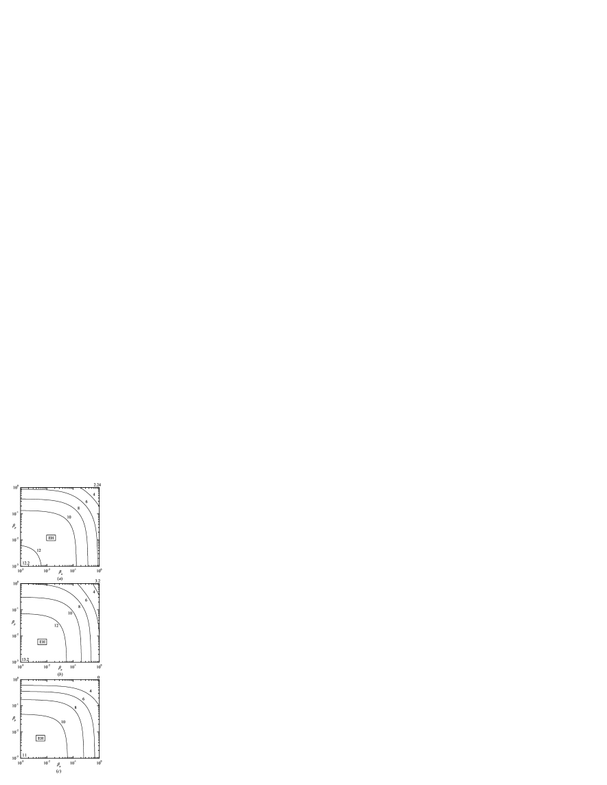
Figure 2: Contour plot of the critical shear rate $a_{c}^{2}$ for Couette flow vs. $\beta_{a}$ and $\beta_{p}$. $a$: $E_{0}=0$; $b$: $E_{0}=E_{F}^{weak}$, $\varepsilon_{a}<0$; $c$: $E_{0}=E_{F}^{weak}$, $\varepsilon_{a}>0$. $E_{F}$ is defined after Eq. (20) and calculated in Eq. (21).

We found that without and with an additional electric field the critical shear rate $a_{c}^{2}$ for the “even” type homogeneous instability (EH) is systematically lower than the threshold for other types of instability (Fig. 2a–c). Note, that in the presence of the field the symmetry with respect to the exchange $\beta_{a}\leftrightarrow\beta_{p}$ is broken.

In Fig. 2 contour plots for the critical value $a_{c}^{2}$ vs. anchoring strengths $\beta_{a}$ and $\beta_{p}$ for different values of the electric field are shown. The differences between $a_{c}^{2}$ obtained from the exact, semi-analytical solution (35) and from the one-mode approximation (42) are indistinguishable in the figure.

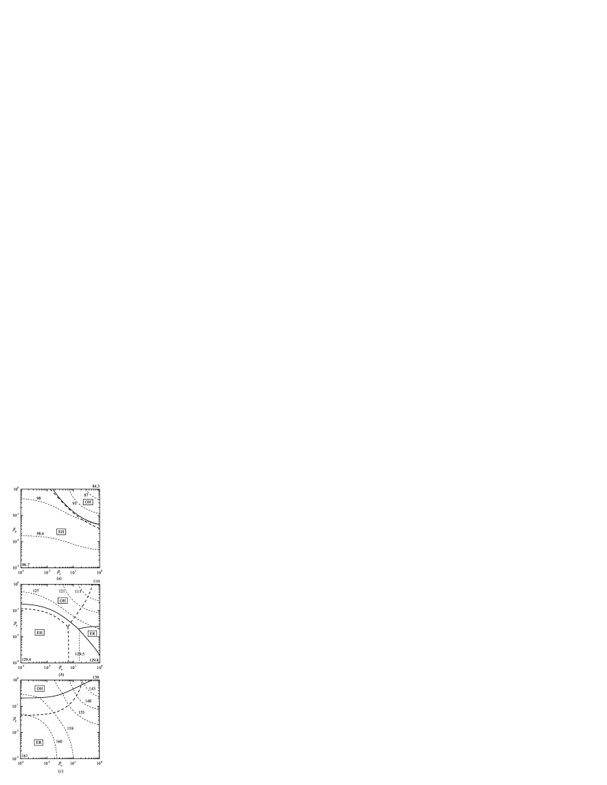
Figure 3: Critical shear rates and phase diagram for the instabilities under Couette flow with additional magnetic field. $a$: $H_{0}/H_{F}=3$; $b$: $H_{0}/H_{F}=3.5$; $c$: $H_{0}/H_{F}=4$. Boundaries for occurrence of instabilities are given by thick solid lines (full numerical) and thick dashed lines (one-mode approximation).

In Fig. 3 contour plots of $a_{c}^{2}$ (thin dashed lines) and the boundaries where the type of instability changes [the solid lines are obtained numerically, the thick dashed lines from (42)] for different values of magnetic field are shown. For not too strong magnetic field in the region of weak anchoring the “odd” type homogeneous instability (OH) takes place (Fig. 3a). Increasing the magnetic field the OH region expands toward stronger anchoring strengths. Above $H_{0}\approx 3.2$ a region with lowest threshold corresponding to the “even” roll mode (ER) appears. This region has borders with both types of the homogeneous instability (Fig. 3b). With increasing magnetic field the ER region increases (Fig. 3c) and above $H_{0}/H_{F}=4$ the ER instability has invaded the whole investigated parameter range. For strong anchoring and $H_{0}/H_{F}=3.5$ the critical wave vector is $q_{c}=5.5$. It increases with increasing magnetic field and decreases with decreasing anchoring strengths. With increasing magnetic field the threshold for the EH instability becomes less sensitive to the surface anchoring. Leslie has pointed out (using an approximate analytical approach) that for strong anchoring a transition from a homogeneous state without transverse flow (EH) to one with such flow (OH) as the magnetic field is increased is not possible in MBBA because of the appearance of the ER type instability Leslie (1976). This is consistent with our results. We find that the EH–OH transition in MBBA is possible only in the region of weak anchoring (Figs. 3a–c).

Figure 4: $a_{c}$ vs. $q$. Couette flow, $\beta_{a}=0.1$, $\beta_{p}=0.1$. $a$: $H_{0}/H_{F}=3$; $b$: $H_{0}/H_{F}=3.4$; $c$: $H_{0}/H_{F}=4$.

In Fig. 4 marginal stability curves for different values of the magnetic field and fixed anchoring strengths is shown (solid line for ER and dashed lines for OR). There are always two minima for the even mode; one of them at $q=0$ that corresponds to the homogeneous instability EH. For small magnetic field the absolute minimum is at $q=0$ (line a). The OR curve is systematically higher than ER. In a small range of $q$ (dotted lines) a stationary ER solution does not exist but we have OR instead. With increasing magnetic field the critical amplitude for the EH minimum ($q=0$) increases more rapidly then the one for the ER minimum ($q\neq 0$) so that for $H_{0}/H_{F}>3.4$ the ER solution is realized (lines b and c). The range of $q$ where ER is replaced by OR expands with increasing magnetic field.

For the ER instability in the absence of fields and strong anchoring we find $a_{c}^{2}=12.15$ from the semi-analytical expression (35) as well as from the one-mode approximation (42) and also (46) with $q=0$. The only available experimental value for $a_{c}^{2}$ is $6.3\pm 0.3$ Pieranski and Guyon (1973). We suspect that the discrepancy is due to deviations from the strong anchoring limit and the difference in the material parameters of the substance used in the experiment. Assuming $\beta_{a}\ll 1$ one would need $\beta_{p}\approx 1$ to explain the experimental value.

V.2 Poiseuille flow

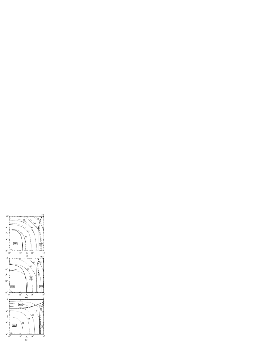
Figure 5: Critical shear rates and phase diagram for the instabilities in Poiseuille flow. $a$: $E_{0}=0$; $b$: $E_{0}=E_{0}^{weak}$, $\varepsilon_{a}<0$; $c$: $E_{0}=E_{0}^{weak}$, $\varepsilon_{a}>0$. Thin dashed lines: full numerical threshold; dotted lines: one-mode approximation for threshold. Boundaries for occurrence of instabilities are given by thick solid lines (full numerical) and thick dashed lines (one-mode approximation).

In Fig. 5 the contour plot for $a_{c}^{2}$ [thin dashed lines from the full numerical calculation, dotted lines from the one-mode approximations (42) and (46)] and the boundary for the various types of instabilities [thick solid line: numerical; thick dashed line: (42) and (46)] are shown. In Poiseuille flow the phase diagram is already very rich in the absence of external fields. In the region of large $\beta_{a}$ one has the EH instability. For intermediate anchoring strengths rolls of type OR occur [Fig. 5$a$]. Note, that even in the absence of the field there is no symmetry under exchange $\beta_{a}\leftrightarrow\beta_{p}$, contrary to Couette flow. The one-mode approximations (42) and (46) not give the transition to EH for strong anchoring. Here we should note that in that region the difference between the EH and the OR instability thresholds is only about 5%. By varying material parameters [increase $\alpha_{2}$ by 10% or decrease $\alpha_{3}$ by 20% or $\alpha_{5}$ by 25% or $K_{33}$ by 35%] it is possible to change the type of instability in that region.

Application of an electric field leads for $\varepsilon_{a}<0$ ($\varepsilon_{a}>0$) to expansion (contraction) of the EH region [Figs. 5$b$ and 5$c$]. At $E_{0}/E_{F}=1$ and $\varepsilon_{a}<0$ rolls vanish completely and the EH instability occurs in the whole area investigated. For $\varepsilon_{a}>0$ the instability of OH type appears in the region of large $\beta_{p}$. In this case, increasing the electric field from $E_{F}^{weak}$ to $E_{F}$ cause an expansion of the OH region. Note that for $\beta_{p}>1$, which is in the OH region, the Freédericksz transition occurs first .

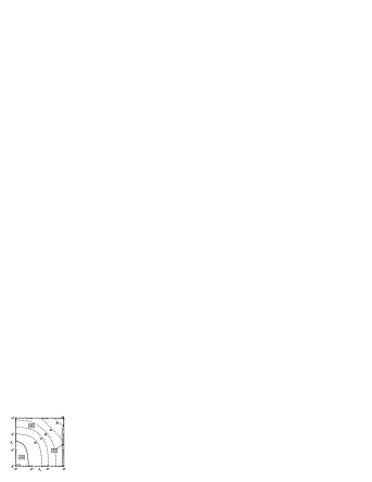
Figure 6: Phase diagram for the instabilities under Poiseuille flow with an additional magnetic field ($H_{0}/H_{F}=0.4$).

An additional magnetic field suppresses the homogeneous instability (Fig. 6). Above $H_{0}/H_{F}\approx 0.5$ the OR instability (Fig. 6) occurs for all anchoring strengths investigated.

The wave vector $q_{c}$ in the absence of fields is $1.4$. Application of an electric field decreases $q_{c}$ whereas the magnetic field increases $q_{c}$. The wave vector decreases with decreasing anchoring strengths.

In the absence of fields and strong anchoring we find for the EH instability $a_{c}=102$ [Eq. (42) gives 110 and Eq. (46) with $q=0$ gives 130]. The experimental value is 92 Guyon and Pieranski (1975). Thus, theoretical calculations and experimental results are in good agreement. Note, that in the experiments Guyon and Pieranski (1975) actually not steady but oscillatory flow with very low frequency was used ($f=5\cdot 10^{-3}$ Hz).

In summary, the orientational instabilities for both steady Couette (semi-analytical for homogeneous instability and numerical for rolls) and Poiseuille flow (numerical) were analysed rigorously taking into account weak anchoring and the influence of external fields. Easy-to-use expressions for the threshold of all possible types of instabilities were obtained and compared with the rigorous calculations. In particular the region in parameter space where the different types of instabilities occurred were determined.

Appendix A Trial functions

In the calculations we used the following set of trial functions:

$$\zeta_{n}^{o}(z;\beta)=\sin(2n\pi z)+2n\pi\beta\sin([2n-1]\pi z),$$

$$\zeta_{n}^{e}(z;\beta)=\cos([2n-1]\pi z)+(2n-1)\pi\beta\cos(2[n-1]\pi z),$$

$$\nu_{n}^{o}(z)=\sin(2n\pi z),\>\nu_{n}^{e}(z)=\cos([2n-1]\pi z),$$

$$\varsigma_{n}^{o}(z)=\dfrac{\sinh(\lambda_{2n}z)}{\sinh(\lambda_{2n}/2)}-\dfrac{\sin(\lambda_{2n}z)}{\sin(\lambda_{2n}/2)},$$

$$\varsigma_{n}^{e}(z)=\dfrac{\cosh(\lambda_{2n-1}z)}{\cosh(\lambda_{2n-1}/2)}-\dfrac{\cos(\lambda_{2n-1}z)}{\cos(\lambda_{2n-1}/2)},$$

$\varsigma_{n}^{o}(z)$ and $\varsigma_{n}^{e}(z)$ are the Chandrasekhar functions and $\lambda_{n}$ are the roots of the corresponding characteristic equations Chandrasekhar (1993).

Appendix B Integrals for the homogeneous instability

B.1 Couette flow

“Odd” solution: $\langle sf\rangle=\langle g\rangle=0$, $\langle f^{2}\rangle=(3+32\beta_{a}+12\pi^{2}\beta_{a}^{2})/6$, $\langle g^{2}\rangle=(3+32\beta_{p}+12\pi^{2}\beta_{p}^{2})/6$, $\langle sfg\rangle=[3+16(\beta_{a}+\beta_{p})+12\pi^{2}\beta_{a}\beta_{p}]/6$, $\langle ff^{\prime\prime}\rangle=-2(3+20\beta_{a}+3\pi^{2}\beta_{a}^{2})/3$, $\langle gg^{\prime\prime}\rangle=-2(3+20\beta_{p}+3\pi^{2}\beta_{p}^{2})/3$.

“Even” solution: $\langle sf\rangle=(2+\pi^{2}\beta_{a})/\pi$, $\langle g\rangle=(2+\pi^{2}\beta_{p})/\pi$, $\langle f^{2}\rangle=(1+8\beta_{a}+2\pi^{2}\beta_{a}^{2})/2$, $\langle g^{2}\rangle=(1+8\beta_{p}+2\pi^{2}\beta_{p}^{2})/2$, $\langle sfg\rangle=[1+4(\beta_{a}+\beta_{p})+2\pi^{2}\beta_{a}\beta_{p}]/2$, $\langle ff^{\prime\prime}\rangle=\pi^{2}(1+4\beta_{a})/2$, $\langle gg^{\prime\prime}\rangle=\pi^{2}(1+4\beta_{p})/2$.

B.2 Poiseuille flow

“Odd” solution: $\langle sf\rangle=-(1+8\beta_{a})/(2\pi)$, $\langle g\rangle=-(2+\pi^{2}\beta_{p})/\pi$, $\langle f^{2}\rangle=(3+32\beta_{a}+12\pi^{2}\beta_{a}^{2})/6$, $\langle g^{2}\rangle=(1+8\beta_{p}+2\pi^{2}\beta_{p}^{2})/2$, $\langle sfg\rangle=-[16+9\pi^{2}(\beta_{a}+\beta_{p})+72\pi^{2}\beta_{a}\beta_{p}]/(18\pi^{2})$, $\langle ff^{\prime\prime}\rangle=-2\pi^{2}(3+20\beta_{a}+3\pi^{2}\beta_{a}^{2})/3$, $\langle gg^{\prime\prime}\rangle=-\pi^{2}(1+4\beta_{p})/2$.

“Even” solution: $\langle sf\rangle=I(g)=0$, $\langle f^{2}\rangle=(1+8\beta_{a}+2\pi^{2}\beta_{a}^{2})/2$, $\langle g^{2}\rangle=(3+32\beta_{p}+12\pi^{2}\beta_{p}^{2})/6$, $\langle sfg\rangle=-[16+9\pi^{2}(\beta_{a}+\beta_{p})+72\pi^{2}\beta_{a}\beta_{p}]/(18\pi^{2})$, $\langle ff^{\prime\prime}\rangle=-\pi^{2}(1+4\beta_{a})/2$, $\langle gg^{\prime\prime}\rangle=-2\pi^{2}(3+20\beta_{p}+3\pi^{2}\beta_{p}^{2})$.

Appendix C Integrals for the spatially periodic instability

C.1 Couette flow

“Odd” solution: $\langle wsf\rangle\approx 0.69043+3.2870\beta_{a}$, $\langle w[sf]^{\prime\prime}\rangle\approx-27.258-32.441\beta_{a}$, $\langle f^{2}\rangle=(3+32\beta_{a}+12\pi^{2}\beta_{a}^{2})/6$, $\langle ff^{\prime\prime}\rangle=-\pi^{2}(6+40\beta_{a}+6\pi^{2}\beta_{a}^{2})/3$, $\langle fsg\rangle=(3+16(\beta_{a}+\beta_{p})+12\pi^{2}\beta_{a}\beta_{p})/6$, $\langle gsu\rangle=(3+16\beta_{p})/6$, $\langle g^{2}\rangle=(3+32\beta_{p}+12\pi^{2}\beta_{p}^{2})/6$, $\langle gg^{\prime\prime}\rangle=-\pi^{2}(6+40\beta_{p}+6\pi^{2}\beta_{p}^{2})/3$, $\langle u^{2}\rangle=1/2$, $\langle uu^{\prime\prime}\rangle=-2\pi^{2}$, $\langle fu\rangle=(3+16\beta_{a})/6$, $\langle w^{2}\rangle=1$, $\langle ww^{\prime\prime}\rangle\approx-46.050$, $\langle ww^{(4)}\rangle=3803.5$, $\langle gw\rangle\approx 0.69043+3.2870\beta_{p}$, $\langle gw^{\prime\prime}\rangle\approx-27.257-32.441\beta_{p}$.

“Even” solution: $\langle wsf\rangle\approx 0.69739+2.6102\beta_{a}$, $\langle w[sf]^{\prime\prime}\rangle\approx-6.8828$, $\langle f^{2}\rangle=(1+8\beta_{a}+2\pi^{2}\beta_{a}^{2})/2$, $\langle ff^{\prime\prime}\rangle=-\pi^{2}(1+4\beta_{a})/2$, $\langle fsg\rangle=(1+4(\beta_{a}+\beta_{p})+2\pi^{2}\beta_{a}\beta_{p})/2$, $\langle gsu\rangle=(1+4\beta_{p})/2$, $\langle g^{2}\rangle=(1+8\beta_{p}+2\pi^{2}\beta_{p}^{2})/2$, $\langle gg^{\prime\prime}\rangle=-\pi^{2}(1+4\beta_{p})/2$, $\langle u^{2}\rangle=1/2$, $\langle uu^{\prime\prime}\rangle=-2\pi^{2}$, $\langle fu\rangle=(1+4\beta_{a})/2$, $\langle w^{2}\rangle=1$, $\langle ww^{\prime\prime}\rangle\approx-12.303$, $\langle ww^{(4)}\rangle\approx 500.56$, $\langle gw\rangle\approx 0.69738+2.6102\beta_{p}$, $\langle gw^{\prime\prime}\rangle\approx-6.8828$.

C.2 Poiseuille flow

“Odd” solution: $\langle wsf\rangle\approx-0.10292-0.49816\beta_{a}$, $\langle w[sf]^{\prime\prime}\rangle\approx-0.87673-22.615\beta_{a}$, $\langle f^{2}\rangle=(3+32\beta_{a}+12\pi^{2}\beta_{a}^{2})/6$, $\langle ff^{\prime\prime}\rangle=-\pi^{2}(6+40\beta_{a}+6\pi^{2}\beta_{a}^{2})/3$, $\langle fsg\rangle=-(16+9\pi^{2}(\beta_{a}+\beta_{p})+72\pi^{2}\beta_{a}\beta_{p})/(18\pi^{2})$, $\langle gsu\rangle=-(16+9\pi^{2}\beta_{p})/(18\pi^{2})$, $\langle g^{2}\rangle=(1+8\beta_{p}+2\pi^{2}\beta_{p}^{2})/2$, $\langle gg^{\prime\prime}\rangle=-\pi^{2}(1+4\beta_{p})/2$, $\langle u^{2}\rangle=1/2$, $\langle uu^{\prime\prime}\rangle=-2\pi^{2}$, $\langle fu\rangle=(3+16\beta_{a})/6$, $\langle w^{2}\rangle=1$, $\langle ww^{\prime\prime}\rangle\approx-12.303$, $\langle ww^{(4)}\rangle\approx 500.56$, $\langle gw\rangle\approx 0.69738+2.6102\beta_{p}$, $\langle gw^{\prime\prime}\rangle\approx-6.8828$.

“Even” solution: $\langle wsf\rangle\approx-0.12206-0.59694\beta_{a}$, $\langle w[sf]^{\prime\prime}\rangle\approx 4.4917$, $\langle f^{2}\rangle=(1+8\beta_{a}+2\pi^{2}\beta_{a}^{2})$, $\langle ff^{\prime\prime}\rangle=-\pi^{2}(1+4\beta_{a})/2$, $\langle fsg\rangle=-(16+9\pi^{2}(\beta_{a}+\beta_{p})+72\pi^{2}\beta_{a}\beta_{p})/(18\pi^{2})$, $\langle gsu\rangle=-(16+9\pi^{2}\beta_{p})/(18\pi^{2})$, $\langle g^{2}\rangle=(3+32\beta_{p}+12\pi^{2}\beta_{p}^{2})/6$, $\langle gg^{\prime\prime}\rangle=-2\pi^{2}(3+20\beta_{p}+3\pi^{2}\beta_{p}^{2})/3$, $\langle u^{2}\rangle=1/2$, $\langle uu^{\prime\prime}\rangle=-\pi^{2}/2$, $\langle fu\rangle=(1+4\beta_{a})/2$, $\langle w^{2}\rangle=1$, $\langle ww^{\prime\prime}\rangle\approx-46.050$, $\langle ww^{(4)}\rangle\approx 3803.5$, $\langle gw\rangle\approx 0.69043+3.2870\beta_{p}$, $\langle gw^{\prime\prime}\rangle\approx-27.257-32.441\beta_{p}$.

References

- Pieranski and Guyon (1974) P. Pieranski and E. Guyon, Phys. Rev. A 9, 404 (1974).
- Pieranski and Guyon (1973) P. Pieranski and E. Guyon, Solid State Communications 13, 435 (1973).
- Dubois-Violette and Manneville (1996) E. Dubois-Violette and P. Manneville, Pattern formation in Liquid Crystals (Springer, New York, 1996), chap. 4.
- Manneville (1979) P. Manneville, Journal de physique 40, 713 (1979).
- Pieranski and Guyon (1976) P. Pieranski and E. Guyon, Communications on Physics 1, 45 (1976).
- Cladis and Torza (1975) P. Cladis and S. Torza, Phys. Rev. Lett. 35, 1283 (1975).
- Nasibullayev et al. (2000) I. Nasibullayev, A. Krekhov, and M. Khazimullin, Mol. Cryst. Liq. Cryst. 351, 395 (2000).
- Nasibullayev and Krekhov (2001) I. Nasibullayev and A. Krekhov, Cryst. Rep. 46, 488 (2001).
- Kedney and Leslie (1998) P. Kedney and F. Leslie, Liquid Crystals 24, 613 (1998).
- Tarasov et al. (2001) O. Tarasov, A. Krekhov, and L. Kramer, Liquid Crystals 28, 833 (2001).
- Chigrinov (1999) V. Chigrinov, Liquid Crystal Devices: Physics and Applications (New York: Artech House, 1999).
- Leslie (1976) F. Leslie, Mol. Cryst. Liq. Cryst. 37, 335 (1976).
- de Gennes (1974) P. G. de Gennes, The physics of liquid crystals (Oxford University Press, 1974).
- Manneville and Dubois-Violette (1976) P. Manneville and E. Dubois-Violette, Journal de Physique 37, 285 (1976).
- (15) Viscosity in units Pa s: , , , , , ; elastic constants in units N: , , ; .
- Guyon and Pieranski (1975) E. Guyon and P. Pieranski, Journal de Physique 36, C1 (1975).
- Chandrasekhar (1993) Chandrasekhar, Hydrodynamic and hydromagnetic instabilities (Montpellier: Capital City Press, 1993).