Abstract

Recently, a continuous dynamics was proposed to simulate dynamics of interpersonal relations in a society represented by a fully connected graph. Final state of such a society was found to be identical with the so-called Heider balance (HB), where the society is divided into two mutually hostile groups. In the continuous model, a polarization of opinions was found in HB. Here we demonstrate that the polarization occurs also in Barabási-Albert networks, where the Heider balance is not necessarily present. In the second part of this work we demonstrate the results of our formalism, when applied to reference examples: the Southern women and the Zachary club.

PACS numbers: 87.23.Ge

Keywords: numerical calculations; sociophysics

1 Introduction

The Heider balance [1, 2, 3, 4, 5] is a final state of personal relations between members of a society, reached when these relations evolve according to some dynamical rules. The relations are assumed to be symmetric, and they can be friendly or hostile. The underlying psycho-sociological mechanism of the rules is an attempt of the society members to remove a cognitive dissonance, which we feel when two of our friends hate each other or our friend likes our enemy. As a result of the process, the society is split into two groups, with friendly relations within the groups and hostile relations between the groups. As a special case, the size of one group is zero, i.e. all hostile relations are removed. HB is the final state if each member interacts with each other; in the frames of the graph theory, where the problem is formulated, the case is represented by a fully connected graph.

Recently a continuous dynamics has been introduced to describe the time evolution of the relations [6]. In this approach, the relations between nodes $i$ and $j$were represented by matrix elements $r(i,j)$, which were real numbers, friendly ($r(i,j)>0$) or hostile ($r(i,j)<0)$. As a consequence of the continuity, we observed a polarization of opinions: the absolute values of the matrix elements $r(i,j)$ increase. Here we continue this discussion, but the condition of maximal connectivity is relaxed, as it could be unrealistic in large societies. The purpose of first part of this work is to demonstrate, that even if HB is not present, the above mentioned polarization remains true. In Section II we present new numerical results for a society of $N=100$ members, represented by Barabási-Albert (BA) network [7]. Although this size of considered social structure is rather small, it is sufficient to observe some characteristics which are different than those in the exponential networks. In second part (Section III) we compare the results of our equations of motion with some examples, established in the literature of the subject. The Section is closed by final conclusions.

2 Calculations for Barabási-Albert networks

The time evolution of $r(i,j)$ is determined by the equation of motion [6]

$$\frac{dr(i,j)}{dt}=\Big{\{}1-\Big{(}\frac{r(i,j)}{R}\Big{)}^{2}\Big{\}}\sum_{k}r(i,k)r(k,j)$$ (1)

where $R$ is a sociologically justified limitation on the absolute value of $r(i,j)$ [6]. Here $R=5.0$. Initial values of $r(i,j)$ are random numbers, uniformly distributed in the range $(-0.5,0.5)$. The equation is solved numerically with the Runge-Kutta IV method with variable length of timestep [8], simultaneously for all pairs $(i,j)$ of linked nodes. The method of construction of BA networks was described in [9]. The connectivity parameter is selected to be $M=7$, because in this case the probability $p(M)$ of HB has a clear minimum for BA networks of $N=100$ nodes, and $p(M=7)\approx 0.5$ (see Fig. 1). This choice of $M$ is motivated by our aim to falsify the result on the polarization of opinions. This polarization was demonstrated [6] to be a consequence of HB; therefore, the question here is if it appears also when HB is not present. An example of time evolution of such a network is shown in Fig. 2.

Our result is that the polarization is present in all investigated cases. As time increases, the distribution of $r(i,j)$ gets wider and finally it reaches a stable shape, with two large peaks at $r(i,j)\approx\pm R$ and one smaller peak at the centre, where $r(i,j)\approx 0$. In Fig. 3, we show a series of histograms of $r(,j)$ in subsequent times (A-E). Particular networks differ quantitatively with respect to the heights of the peaks, but these differences are small.

We note here that when some links are absent, the definition of HB should be somewhat relaxed, because some other links, which do not enter to any triad $(i,j,k)$, will not evolve at all. Therefore we should admit that some negative relations survive within a given group. We classify a final state of the graph as HB if there are no chains of friendly relations between the subgroups. On the other hand, more than two mutually hostile subgroups can appear. These facts were recognized already in literature [3, 5]. Surprisingly enough, subgroups of $1<N<97$ nodes are never found in our BA networks. On the contrary, in the exponential networks groups of all sizes were detected. In Figs. 4 and 5 we show diagrams for BA networks and exponential networks, respectively. Each point at these diagrams marks the value of $r(i,j)$ and the size of the subgroup which contains nodes $(i,j)$. Links between different subgroups are omitted. We see that for BA networks (Fig.4), the lowest value of $N$ is 97. The remaining three nodes are linked with all other nodes by hostile relations.

3 Examples

In Ref. [6], an example of polarization of opinions on the lustration law in Poland in 1999 was brought up. The presented statistical data [10] displayed two maxima at negative and positive opinions and a lower value at the centre of the plot. In our simulations performed for fully connected graphs [6], the obtained value for the center was zero. However, it is clear that in any group larger than, say, 50 persons some interpersonal relations will be absent. Taking this into account, we can claim than the statistical data of [10] should be compared to the results discussed here rather than to those for a fully connected graph. Here we reproduce a peak of the histogram at its centre, on the contrary to the results in [6]. This fact allows to speak on a qualitative accordance of the results of our calculations with the statistical data of [10].

Next example is the set of data of the attendance of 18 ’Southern women’ in local meetings in Natchez, Missouri, USA in 1935 [11]. These data were used to compare 21 methods of finding social groups. The results were analysed with respect to their consensus, and ranked with consensus index from 0.543 (much worse than all others) to 0.968. To apply our dynamics, we use the correlation function $<p(i,j)>-<p(i)><p(j)>$ as initial values of $r(i,j)$. Our method produced the division (1-9) against (10-18), what gives the index value 0.968. As a by-product, the method can provide the time dynamics of the relations till HB and, once HB is reached, the leadership within the cliques [12]. We should add that actually, we have no data on the possible friendship or hostility between these women, then the interpretation of these results should be done with care.

Last example is the set of data about a real conflict in the Zachary karate club [13, 14, 15]. The input data are taken from [16]. All initial values of the matrix elements are reduced by a constant $\epsilon$ to evade the case of overwhelming friendship. The obtained splitting of the group is exactly as observed by Zachary: (1-8,11-14,17,18,20,22) against (9,10,15,16,19,21,23-34). These results were checked not to vary for $\epsilon$ between 1.0 and 3.0. The status of all group members can be obtained with the same method as in the previous example.

To conclude, the essence of Eq. (1) is the nonlinear coupling between links $r(i,j)$, which produces the positive feedback between the actual values of the relations and their time evolution. We should add that the idea of such a feedback is not entirely new. It is present, for example, in Boltzmann-like nonlinear master equations applied to behavioral models [17]. On the contrary, it is absent in later works on formal theory of social influence [18]. On the other hand, the theories of status [12] are close to the method of transition matrix, known in non-equilibrium statistical mechanics [19].

Figure 1: The number of networks per 1000 trials, where HB is not reached.

Figure 2: The number of unbalanced triangles of nearest neighbours $(i,j,k)$ against time. Six successive times for Fig. 3 are marked with labels A-F.

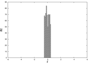
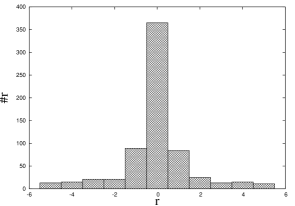
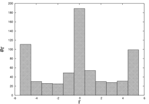
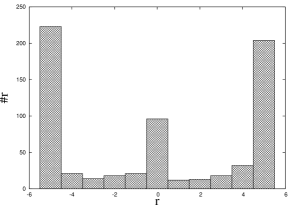
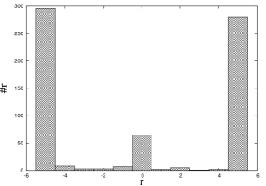
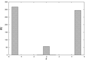
Figure 3: Time evolution of the histogram of the matrix elements $r(i,j)$.

Figure 4: Diagram of values of $r(i,j)$ and the group size for BA networks.

Figure 5: Diagram of values of $r(i,j)$ and the group size for exponential networks.

References

- [1] F. Heider, J. of Psychology 21 (1946) 107.
- [2] F. Heider, The Psychology of Interpersonal Relations, J.Wiley and Sons, New York 1958.
- [3] F. Harary, R. Z. Norman and D. Cartwright, Structural Models: An Introduction to the Theory of Directed Graphs, John Wiley and Sons, New York 1965.
- [4] P. Doreian and A. Mrvar, Social Networks 18 (1996) 149.
- [5] Z. Wang and W. Thorngate, J. of Artificial Societies and Social Simulation, Vol 6, No 3 (2003).
- [6] K. Kułakowski, P. Gawroński and P. Gronek, Int. J. Mod. Phys. C (2005), in print (physics/0501073) See also (physics/0501160).
- [7] R. Albert and A.-L. Barabási, Rev. Mod. Phys. 286 (2002) 47.
- [8] M. Abramowitz and I. A. Stegun (Eds.), Handbook of Mathematical Functions, Dover, New York, 1972.
- [9] K. Malarz and K. Kułakowski, Physica A 345 (2005) 326 (see also cond-mat/0501545).
- [10] Report BS/152/99 of the Public Opinion Research Center, Tab. 3 (in Polish).
- [11] L. C. Freeman, in R. Breiger, K. Carley and P. Pattison (Eds.), Dynamic Social Network Modeling and Analysis, Washington, D.C.:The National Academies Press, 2003.
- [12] Ph. Bonacich and P. Lloyd, Social Networks 23 (2001) 191.
- [13] W. W. Zachary, J. Anthrop. Res. 33 (1977) 452.
- [14] L. Donetti and M. Muñoz, J. Stat. Mech.: Theor. Exp. (2004) 10012.
- [15] M. Girvan and M. E. J. Newman, Phys. Rev. E 69 (2004) 026113.
- [16] vlado.fmf.uni-lj.si/pub/networks/data/Ucinet/UciData.htm, dataset ZACHC
- [17] D. Helbing, Physica A 196 (1993) 546.
- [18] N. E. Friedkin and E. C. Johnsen, Social Networks 19 (1997) 209.
- [19] L. E. Reichl, A Modern Course in Statistical Physics, J. Wiley and Sons, New York 1998, p. 241.