Systematic analysis of group identification in stock markets

Abstract

We propose improved methods to identify stock groups using the correlation matrix of stock price changes. By filtering out the marketwide effect and the random noise, we construct the correlation matrix of stock groups in which nontrivial high correlations between stocks are found. Using the filtered correlation matrix, we successfully identify the multiple stock groups without any extra knowledge of the stocks by the optimization of the matrix representation and the percolation approach to the correlation-based network of stocks. These methods drastically reduce the ambiguities while finding stock groups using the eigenvectors of the correlation matrix.

I Introduction

The study of correlations in stock markets has attracted much interest of physicists because of its challenging complexity as a complex system and its possible future applications to the real markets book . In the early years, a correlation-based taxonomy of stocks and stock market indices was studied by the method of the hierarchical tree Mantegna ; Bonanno1 . Recently, the minimum spanning tree technique was introduced to study the structure and dynamics of the stock network Bonanno2 ; Onnela1 ; Onnela2 , the random matrix theory was applied to find out the difference between the random and nonrandom property of the correlations Laloux ; Plerou1 ; Plerou2 ; Gopikrishnan ; Utsugi , and the maximum likelihood clustering method was developed and applied to identify cluster structures in stock markets Giada . Also, these studies have been extended to the applications to the portfolio optimization in real market Plerou2 ; Onnela1 .

Commonly, the correlation between stocks is expressed by the Pearson correlation coefficient of log-returns,

$$G_{i}(t)\equiv\ln S_{i}(t+\Delta t)-\ln S_{i}(t),$$ (1)

where $S_{i}(t)$ is the price of stock $i$ at time $t$. From real time series data of $N$ stock prices, we can calculate the element of $N\times N$ correlation matrix $\mathbf{C}$ as following

$$C_{ij}=\frac{\langle(G_{i}(t)-\langle G_{i}\rangle)(G_{j}(t)-\langle G_{j}\rangle)\rangle}{\sqrt{(\langle G_{i}^{2}\rangle-\langle G_{i}\rangle^{2})(\langle G_{j}^{2}\rangle-\langle G_{j}\rangle^{2})}},$$ (2)

where $\langle\cdots\rangle$ indicates time averages over the period of the time series. By definition, $C_{ii}=1$ and $C_{ij}$ has a value in $[-1,1]$.

Laloux et al. Laloux and Plerou et al. Plerou1 ; Plerou2 studied the statistical properties of an empirical correlation matrix between stock price changes defined in Eq. (2) for real markets. In comparison with the prediction of the random matrix theory, they found that the statistics of the bulk eigenvalues are in remarkable agreements with the universal properties of the random correlation matrix. For example, the bulk part of the eigenvalue spectrum of the empirical correlation matrix for $N$ stocks over $L$ price data has the form of the spectrum of the random correlation matrix Sengupta which is given by

$$\rho(\lambda)=\frac{Q}{2\pi}\frac{\sqrt{(\lambda_{max}-\lambda)(\lambda-\lambda_{min})}}{\lambda},$$ (3)

for $\lambda\in[\lambda_{min},\lambda_{max}]$ in the limit of $N,L\to\infty$ with fixed $Q\equiv L/N$, where $\lambda_{max}=(1+1/\sqrt{Q})^{2}$ and $\lambda_{min}=(1-1/\sqrt{Q})^{2}$. Moreover, the level spacing statistics of eigenvalues exhibits good agreement with the results from the Gaussian orthogonal ensemble of random matrices Plerou1 ; Plerou2 .

On the other hand, the nonrandom properties of the correlation matrix have also been studied with the empirical correlation matrix Plerou1 ; Plerou2 ; Gopikrishnan . From the empirical data for the New York Stock Exchange, it was found that each eigenvector corresponding to the few largest eigenvalues larger than the upper bound of the bulk eigenvalue spectrum, is $\it localized$, in a sense that only a few components contribute to the eigenvector mostly, and the stocks corresponding to those dominant components of the eigenvector are found to belong to a common industry sector. Very recently, Utsugi et al. confirmed and improved those results through the similar analysis for the Tokyo Stock Exchange Utsugi .

Figure 1: The normalized eigenvector components $u_{i}(\lambda)$ of stock $i$ corresponding to the second to fifth largest eigenvalues $\lambda_{1}$ - $\lambda_{4}$ of the correlation matrix. The stocks are sorted by industrial sectors, A: basic materials, B: capital goods, C: conglomerates, D: consumer (cyclical), E: consumer (noncyclical), F: energy, G: financial, H: healthcare, I: services, J: technology, K: transportation, and L: utilities, which are separated by dashed lines.

In order to confirm the localization property of eigenvectors, we perform the similar analysis to the previous studies Plerou1 ; Plerou2 ; Gopikrishnan on eigenvectors of the correlation matrix using our own dataset of stock prices. We analyze the daily prices of $N=135$ stocks belonging to the New York Stock Exchange (NYSE) for the 20-year period $1983-2003$ ($L\simeq 5000$ trading days) which is publicly available from the web-site(http://finance.yahoo.com) comment0 . Indeed, if we put stocks in the order of their industrial sectors, we observe that the eigenvector components corresponding to stocks which belong to specific industrial sectors give high contributions to each of the eigenvectors for the few largest eigenvalues (see Fig. 1). For instance, the stocks belonging to the energy, technology, transportation, and utilities sectors highly contribute to the eigenvector for the second largest eigenvalue; the energy sector constitutes the big part of the eigenvector for the third largest eigenvalue; the fourth largest eigenvalue gives the eigenvector localized on the basic materials, consumer (noncyclical), healthcare, and utilities sectors; the eigenvector for the fifth largest eigenvalue is also localized on several specific industrial sectors.

However, it is not straightforward to find out specific stock groups, such as the industrial sectors, inversely. If each of the eigenvectors had well-defined dominant components and the corresponding set of stocks were independent of the sets from other eigenvectors, it would become easy to identify the stock groups. Unfortunately, in our study, it turns out that not only the set of eigenvector components with dominant contribution can be hardly defined in the eigenvector but also such a set is likely to overlap with the sets from other eigenvectors unless we pick a very small number of stocks with few highest ranks of their contributions to the eigenvectors; Figure 1 indicates that each of the eigenvectors is localized on a multiple number of industrial sectors and the corresponding stocks severely overlap with those from the other eigenvectors. Therefore it is very ambiguous to identify the stock groups for practical purposes. The aim of this study is to get rid of these ambiguities and finally find out relevant stock groups without any aid of the table of industrial sectors.

In this paper, we introduce the improved method to identify stock groups which drastically reduce the ambiguities in finding multiple groups using eigenvectors of the correlation matrix. We first filter out the random noise and the marketwide effect from the correlation matrix. With the filtered correlation matrix, we apply optimization and percolation approaches to find the stock groups. Through the optimization of the stock sequences representing the matrix indices, the filtered correlation matrix is transformed into the block diagonal matrix in which all stocks in a block are found to belong to the same group. By constructing a network of stocks using the percolation approach on the filtered correlation matrix, we also successfully identify the stock groups which appear in the form of isolated clusters in the resulting network.

This paper is organized as follows. In Sec. II, the detailed filtering method to construct the group correlation matrix is given. For the filtering, the largest eigenvalue and the corresponding eigenvector are required and they are calculated from the first-order perturbation theory. In Sec. III, detailed stock group finding methods using the optimization and the percolation are given and the resulting stock groups are specified. In Sec. IV, a summary and conclusions are presented.

II Group correlation matrix

II.1 Filtering

The group of stocks is defined as a set of highly intercorrelated stocks in their price changes. In the empirical correlation matrix, because several types of noises are expected to coexist with the intragroup correlations, it is essential to filter out such noises to isolate the intragroup correlations which we are interested in. With the complete set of eigenvalues and eigenvectors, the correlation matrix in Eq. (2) can be expanded as

$$\mathbf{C}=\sum^{N-1}_{\alpha=0}\lambda_{\alpha}|\alpha\rangle\langle\alpha|,$$ (4)

where $\lambda_{\alpha}$ is the eigenvalue sorted in descending order and $|\alpha\rangle$ is the corresponding eigenvector. Because only the eigenvectors corresponding to the few largest eigenvalues are believed to contain the information on significant stock groups, we can identify a filtered correlation matrix for stock groups by choosing a partial sum of $\lambda_{\alpha}|\alpha\rangle\langle\alpha|$ relevant to stock groups, which we will call the group correlation matrix, $\mathbf{C}^{g}$.

In order to extract $\mathbf{C}^{g}$ from the correlation matrix, taking the previous results of Plerou et al.  Gopikrishnan ; Plerou1 ; Plerou2 for granted, we posit that the eigenvalue spectrum of the correlation matrix is organized by the marketwide part of the largest eigenvalue, the group part of intermediate discrete eigenvalues, and the random part of small bulk eigenvalues. Then, we can separate the correlation matrix into three parts as

$$\mathbf{C} = \mathbf{C}^{m}+\mathbf{C}^{g}+\mathbf{C}^{r}$$ (5)

$$= \lambda_{0}|0\rangle\langle 0|+\sum^{N_{g}}_{\alpha=1}\lambda_{\alpha}|\alpha\rangle\langle\alpha|+\sum^{N-1}_{\alpha=N_{g}+1}\lambda_{\alpha}|\alpha\rangle\langle\alpha|,$$

where $\mathbf{C}^{m}$, $\mathbf{C}^{g}$, and $\mathbf{C}^{r}$ indicate the marketwide effect, the group correlation matrix, and the random noise terms, respectively.

Figure 2: (a) The eigenvalues $\lambda>1.0$ of the correlation matrix $\mathbf{C}$ and (b) the distribution of bulk eigenvalues $P(\lambda)$ (solid line). The dashed-dot line marks our boundary between the random noise part and the group correlation part. (c) The matrix element distribution for the group correlation matrix $\mathbf{C}^{g}$ and the residual parts corresponding to the bulk eigenvalues $\mathbf{C}^{r}$ and the largest eigenvalue $\mathbf{C}^{m}$.

While the determination of $\mathbf{C}^{m}$ is straightforward, it is not so clear to determine $N_{g}$ for separating $\mathbf{C}^{g}$ and $\mathbf{C}^{r}$. If there were no correlation between stock prices, the bulk eigenvalues have to follow Eq. (3), and thus the upper bound of the bulk eigenvalues can be clearly determined from $Q$. However, in empirical correlation matrix, the bulk eigenvalue spectrum deviates from Eq. (3) due to the coupling with underlying structured correlations, such as the group correlation embedded in $\mathbf{C}^{g}$ Burda . Therefore we use a graphical estimation to determine $N_{g}$; in the eigenvalue spectrum as shown in Fig. 2(b) we choose the cut $N_{g}=9$ in the vicinity of the blurred tail of the bulk part of the spectrum. Nevertheless, in spite of the rough estimation of $N_{g}$, we note that our results in this work do not alter from a small change of $N_{g}$, $\sim\pm 1$. This can be justified by the following arguments. In the group correlation matrix, the corresponding component of the eigenvalues close to the bulk part of the spectrum is confined to only a very small portion of the whole matrix; because the elements of the correlation matrix component $\lambda_{\alpha}|\alpha\rangle\langle\alpha|$ must be smaller than the eigenvalue $\lambda_{\alpha}$, large discrete eigenvalues dominantly contribute to the group correlation matrix. In addition, even if we count one less eigenvalue near the boundary of bulk part of the spectrum in constructing the group correlation matrix, a possible information loss of groups is not likely serious because the pure eigenvectors of the groups generally turn out to be mixed all together in the eigenvectors of the correlation matrix (see Fig. 1). Therefore the influence from the error in the determination of $N_{g}$ is insignificant so that it does not change the clustering result.

This decomposition of the correlation matrix gives nontrivial characteristics to the distribution of the group correlation matrix elements $C^{g}_{ij}$. In Fig. 2(c), it turns out that the distribution of $C^{g}_{ij}$ shows positive heavy tail. This indicates that $\mathbf{C}^{g}$ contains a non-negligible number of strongly correlated stock pairs, which is expected to come from the correlation between the stocks belonging to the same group. On the other hand, $\mathbf{C}^{r}$ shows the Gaussian distribution consistent with the prediction of the random matrix theory Plerou2 . While this Gaussian-like distribution is also observed partially in the distribution of $C^{g}_{ij}$ due to the coupling between group correlations and random noises, it turns out that this remaining noise does not seriously affect the identification of stock groups. The distribution of $C^{m}_{ij}$ shows that $\mathbf{C}^{m}$ also contains highly correlated stock pairs, but we find that $C^{m}_{ij}$ is not relevant to the group correlation and thus have to be filtered out for the clear identification of the stock groups, which is discussed in Sec. II.2.

Figure 3: The $Q\equiv L/N$ dependence of the matrix element distribution for $\mathbf{C}^{g}$ (thick solid line), $\mathbf{C}^{r}$ (solid line), and $\mathbf{C}^{m}$ (dashed line). With fixed $N=135$, various time periods are tested for (a) $L\simeq 2600$ ($1993-2003$), (b) $L\simeq 950$ ($2000-2003$), and (c) $L\simeq 240$ ($2003$).

Since the quality of the correlation matrix can depend on the period of empirical data or generally $Q\equiv L/N$, our decomposition of the correlation matrix can also depend on $Q$. Here we simply check how the determination of $N_{g}$ and the resulting matrix element distribution of the decomposed matrices are changed depending on $Q$ (see Fig. 3). For $Q=19.4$ ($1993-2003$) and $Q=7.0$ ($1999-2003$), $\mathrm{C}^{g}$ and $\mathrm{C}^{r}$ are separated at $N_{g}=10$, which is not very different from $N_{g}=9$ of the larger dataset we use throughout this paper, and in addition, the distribution of the matrix element shows the similar degree of the heavy tail in $C^{g}_{ij}$. However, decreasing $Q$ much smaller, the bulk eigenvalue spectrum becomes wider so that more eigenvalues relevant to the group correlation can be buried in the bulk spectrum, which leads to smaller $N_{g}$ that turns to be $7$ for $Q=1.7$ (2003). Even in this case of $Q=1.7$, the positive heavy tail is still found in $C^{g}_{ij}$ but very weaker than higher $Q$’s. These imply that we need a large enough $Q$ for the stock group identification.

II.2 Largest eigenvalue and corresponding eigenvector

Our filtering is based on the following interpretations of the previous studies: the bulk part of the eigenvalues and their eigenvectors are expected to show the universal properties of the random matrix theory and the largest eigenvalue and its eigenvector are considered as a collective response of the entire market Plerou1 ; Plerou2 ; Gopikrishnan . While the random characteristics of the bulk eigenvalues have been studied intensively, only the empirical tests have been done for the largest eigenvalue and its eigenvector so far Plerou2 ; Gopikrishnan . Thus, to understand the more accurate meaning, we calculate the largest eigenvalue and its eigenvector of the correlation matrix by using perturbation theory.

In stock markets, it has been understood that there exist three kinds of fluctuations in stock price changes: a marketwide fluctuation, synchronized fluctuations of stock groups, and a random fluctuation Plerou1 ; Plerou2 ; Gopikrishnan . For simplicity, we consider a situation in which a system with only the marketwide fluctuation is perturbed by other fluctuations. Let us assume that the price changes of all the stocks in the market find a synchronized background fluctuation with zero mean and variance $c_{0}$ as a marketwide effect. Then, we can write down the $N\times N$ unperturbed correlation matrix as

$$\mathbf{C}^{0}=\left(\begin{array}[]{cccc}1&c_{0}&\cdots&c_{0}\\ c_{0}&1&&\vdots\\ \vdots&&\ddots&c_{0}\\ c_{0}&\cdots&c_{0}&1\end{array}\right),$$ (6)

which has the largest eigenvalue $\lambda^{(0)}_{0}=c_{0}(N-1)+1$ and its eigenvector components $u^{(0)}_{i}=\langle(stock)~{}i|0^{(0)}\rangle=1/\sqrt{N}$.

When a small perturbation is turned on, the total correlation matrix becomes

$$\mathbf{C}=\mathbf{C}^{0}+\mathbf{\Delta},$$ (7)

where $\Delta_{ii}=0$ and $\Delta_{ij}=\Delta_{ji}$. Applying the perturbation theory up to the first order, the largest eigenvalue and the corresponding eigenvector components are easily calculated as

$$\lambda_{0} = c_{0}(N-1)+1+\frac{1}{N}\sum_{i,j}\Delta_{ij},$$

$$u_{i} = \frac{1}{c_{0}N^{3/2}}\left(w_{i}+c_{0}-\frac{1}{N}\sum_{j,k}\Delta_{jk}\right),$$ (8)

where $w_{i}=\sum_{j\neq i}C_{ij}$.

We check the validity of Eqs. (II.2) by comparing with the largest eigenvector obtained from the numerical diagonalization of the empirical correlation matrix. For the comparison, we make the distribution of $C_{ij}$ in Eq. (7) to be close to the empirical $C_{ij}$ distribution by assuming that $\Delta_{ij}$ follows the bell-shaped distribution with zero mean and letting $c_{0}$ to the mean value of the empirical $C_{ij}$. Because the assumption not only reproduces the distribution of empirical $C_{ij}$, but also allows us to neglect the $1/N\sum\Delta_{ij}$ term in Eqs. (II.2), we can directly compare the perturbation theory with the numerical result. Figure 4 displays the eigenvector components of the largest eigenvalue obtained from the empirical correlation matrix and the dominant terms of Eqs. (II.2), which show remarkable agreement with each other.

Figure 4: The comparison of the eigenvector of the largest eigenvalue obtained by the exact diagonalization $u_{i}$ and the dominant term $(w_{i}+c_{0})/(c_{0}N^{3/2})$ in Eq. (II.2). The dashed line has the slope $1.0$. (Inset: the values of corresponding eigenvector components.)

Equation (II.2) indicates that the eigenvector of the largest eigenvalue is contributed by not only the global fluctuation but also the unknown perturbations from $\mathbf{\Delta}$ including random noises. Thus, by filtering out the $\mathbf{C}^{m}$ term, we can decrease the effect of unnecessary perturbations in constructing the group correlation matrix. Indeed, as seen in Fig. 2(c), because the heavy tail part of $\mathbf{C}^{g}$, the highly correlated elements, are buried in $\mathbf{C}^{m}$, the clustering of stocks would be seriously disturbed unless $\mathbf{C}^{m}$ is filtered out.

In addition, Eqs. (II.2) also enable us to interpret more detailed meaning of the eigenvector than the marketwide effect. Because the $i$th eigenvector component $u_{i}$ is mostly determined by $w_{i}$, the sum of the correlation over all the other stocks, it can be regarded as the influencing power of the company in the entire stock market. In real data, the top four stocks with highest $w_{i}$ are found to be General Electric (GE), American Express (AXP), Merrill Lynch (MER), and Emerson Electric (EMR), mostly conglomerates or huge financial companies, which convinces us that $u_{i}$ is indeed representing the influencing power of stock $i$. However, these high influencing companies prevent clear clustering of stocks because of their non-negligible correlations with entire stocks in the market. This is easily comprehensible by considering an analogous situation in a network where the big hub, a node with a large number of links, can make indispensable connections between groups of nodes to cause difficulties in distinguishing the groups Holme . Therefore it is very important to filter out $\mathbf{C}^{m}$ in order to identify the groups of stocks efficiently.

III Identification of stock groups

In the group model for stock price correlation proposed by Noh Noh , the correlation matrix $\mathbf{C}$ takes the form of $\mathbf{C}=\mathbf{C}^{g}+\mathbf{C}^{r}$, where $\mathbf{C}^{g}$ and $\mathbf{C}^{r}$ are the correlation matrix of stock groups and random correlation matrix, respectively. The model assumes the ideal situation with $C^{g}_{ij}=\delta_{\alpha_{i},\alpha_{j}}$, where $\alpha_{i}$ indicates the group to which the stock $i$ belongs. Thus $\mathbf{C}^{g}$ is the block diagonal matrix,

$$\mathbf{C}^{g}=\left(\begin{array}[]{cccc}\mathbf{1}_{0}&0&\cdots&0\\ 0&\mathbf{1}_{1}&&\vdots\\ \vdots&&\ddots&0\\ 0&\cdots&0&\mathbf{1}_{n}\end{array}\right),$$ (9)

where $\mathbf{1}_{i}$ is the $N_{i}\times N_{i}$ matrix ($N_{i}$ is the number of stocks in the $i$th group) of which all elements are $1$.

Here we use this group model to find the groups of stocks. If the correlation matrix in the real market can be represented by the block diagonal matrix as in the model, it would be very easy to identify the groups of stocks. However, there exist infinitely many possible representations of the matrix depending on indexing of rows and columns even if we have a matrix equivalent to the block diagonal matrix. For instance, if we exchange the indices of the matrix (e.g., $\{i,j,k\}\to\{k,i,j\}$) the matrix may not be block-diagonal anymore. Therefore the problem in identifying the groups in stock correlation matrix requires one to find out the optimized sequence of stocks to transform the matrix into the well-organized block diagonal matrix comment1 .

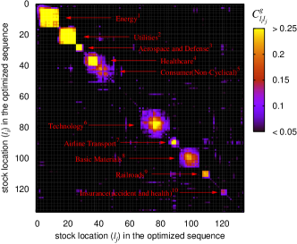
Figure 5: (Color online) The visualization of the group correlation matrix with the optimized stock sequence $\{l_{i}\}$.

To optimize the sequence of stocks for clear block diagonalization, we consider the correlation between two stocks as an attraction force between them. For the ideal group correlation matrix in the group model, the block diagonal form is evidently the most stable form if the attractive force between stocks is proportional to their correlation within the group. To deal with the real correlation matrix, we define the total energy for a stock sequence as

$$E_{tot}=\sum_{i<j}C^{g}_{ij}|l_{i}-l_{j}|\Theta(C^{g}_{ij}-c_{c}),$$ (10)

where $l_{i}$ is the location of the stock $i$ in the new index sequence and the cutoff $c_{c}=0.1$ is introduced to get rid of the random noise part which still remains in $\mathbf{C}^{g}$ in spite of the filtering comment2 .

Figure 6: The dependence of the number of isolated clusters, $m$, in the stock network on the threshold $p$ in constructing the network from (a) the group correlation matrix and (b) the full correlation matrix.

We obtain the optimized sequence of stocks to minimize the total energy defined in Eq. (10) by using the simulated annealing technique Kirkpatrick in Monte Carlo simulation. The following description of our problem is very similar to the well-known traveling salesman problem, finding an optimized sequence of visiting cities which minimizes total traveling distance nr :

1. Configuration. The stocks are numbered $i=0,\ldots,N-1$. A configuration, a sequence of stocks $\{l_{i}\}$, is a permutation of the numbers $0,\ldots,N-1$.

2. Rearrangements. A randomly chosen stock in the sequence is removed and inserted at the random position of the sequence.

3. Objective function. We use $E_{tot}$ in Eq. (10) as an objective function to be minimized after rearrangements.

Table 1: The full list of the optimized sequence of stocks. The footnotes correspond to the identified stock groups represented by the same footnotes in Fig. 5.

$p_{i}$	Ticker	Sector	$p_{i}$	Ticker	Sector	$p_{i}$	Ticker	Sector
0	XNR	Services	45	G	Consumer noncyclical5	90	AMR	Transportation7
1	WMB	Utilities	46	AVP	Consumer noncyclical5	91	F	Consumer cyclical7
2	VLO	Energy1	47	MCD	Services	92	GM	Consumer cyclical7
3	NBL	Energy1	48	IFF	Basic materials	93	HPC	Basic materials8
4	APA	Energy1	49	WMT	Services	94	DD	Basic materials8
5	KMG	Energy1	50	FNM	Financial	95	CAT	Capital goods8
6	HAL	Energy1	51	EC	Consumer cyclical	96	DOW	Basic materials8
7	SLB	Energy1	52	KR	Services	97	WY	Basic materials8
8	BP	Energy1	53	HET	Services	98	IP	Basic materials8
9	COP	Energy1	54	TXI	Capital goods	99	GP	Basic materials8
10	CVX	Energy1	55	FO	Conglomerates	100	BCC	Basic materials8
11	OXY	Energy1	56	SKY	Capital goods	101	AA	Basic materials8
12	RD	Energy1	57	FLE	Capital goods	102	PD	Basic materials8
13	MRO	Energy1	58	RSH	Services	103	LPX	Basic materials8
14	XOM	Energy1	59	EK	Consumer cyclical	104	N	Basic materials8
15	PGL	Utilities2	60	EMR	Conglomerates	105	DE	Capital goods
16	CNP	Utilities2	61	TOY	Services	106	PBI	Technology
17	ETR	Utilities2	62	TEN	Consumer cyclical	107	BDK	Consumer cyclical
18	DTE	Utilities2	63	ROK	Technology	108	UNP	Transportation9
19	EXC	Utilities2	64	HON	Capital goods	109	NSC	Transportation9
20	AEP	Utilities2	65	AXP	Financial	110	CSX	Transportation9
21	PEG	Utilities2	66	GRA	Basic materials	111	BNI	Transportation9
22	SO	Utilities2	67	VVI	Services	112	CNF	Transportation9
23	ED	Utilities2	68	CSC	Technology6	113	MAT	Consumer cyclical
24	PCG	Utilities2	69	DBD	Technology6	114	C	Financial
25	EIX	Utilities2	70	HRS	Technology6	115	VIA	Services
26	LMT	Capital goods3	71	STK	Technology6	116	MMM	Conglomerates
27	NOC	Capital goods3	72	ZL	Technology6	117	DIS	Services
28	RTN	Conglomerates3	73	TEK	Technology6	118	BC	Consumer cyclical
29	GD	Capital goods3	74	AVT	Technology6	119	CBE	Technology
30	BA	Capital goods3	75	GLW	Technology6	120	THC	Healthcare10
31	BOL	Healthcare4	76	NSM	Technology6	121	HUM	Financial10
32	MDT	Healthcare4	77	TXN	Technology6	122	AET	Financial10
33	BAX	Healthcare4	78	MOT	Technology6	123	CI	Financial10
34	WYE	Healthcare4	79	HPQ	Technology6	124	JCP	Services
35	BMY	Healthcare4	80	NT	Technology6	125	MEE	Energy
36	LLY	Healthcare4	81	IBM	Technology6	126	GE	Conglomerates
37	MRK	Healthcare4	82	UIS	Technology6	127	UTX	Conglomerates
38	PFE	Healthcare4	83	XRX	Technology6	128	R	Services
39	JNJ	Healthcare4	84	T	Services	129	NVO	Healthcare
40	PEP	Consumer noncyclical5	85	HIT	Capital goods	130	GT	Consumer cyclical
41	KO	Consumer noncyclical5	86	MER	Financial	131	S	Services
42	PG	Consumer noncyclical5	87	FDX	Transportation7	132	NAV	Consumer cyclical
43	MO	Consumer noncyclical5	88	LUV	Transportation7	133	CEN	Technology
44	CL	Consumer noncyclical5	89	DAL	Transportation7	134	FL	Services

Figure 5 visualizes the correlation matrix elements $C^{g}_{l_{i}l_{j}}$ with the most optimized sequence $\{l_{i}\}$ and Table 1 lists the optimized sequence of stocks. The multiple independent blocks of highly correlated correlations in the matrix are clearly visible without any a priori knowledge of stocks, i.e., the stocks in different blocks are believed to belong to different groups. We succeed to identify about $70\%$ of the entire $135$ stocks from the blocks, which are listed in Table 1 and it turns out that most of the stocks in a block are represented by a single industry sector or a detailed industrial classification such as aerospace and defense, airline transport, railroad, and insurance (see Fig. 5). There still remain a small number of ungrouped stocks, which arises from the fact that the correlations between them are too weak to be distinguished from the random noise that still exists in the group correlation matrix.

As an alternative method, we also perform a network-based approach to find the groups of stocks. In principle, the correlation matrix can be treated as an adjacency matrix of the weighted network of stocks, in which the weights indicate how closely correlated the stocks are in their price changes Swson . However, for the simplicity and the clear definition of groups in the network, we consider the binary network of stocks which permits only two possible states of a stock pair, connected or disconnected.

To construct the binary network of stocks, we use the percolation approach because of its usefulness of finding groups. The method is very simple: for each pair of stocks, we connect them if the group correlation coefficient $C^{g}_{ij}$ is larger than a preassigned threshold value $p$. If the heavy tail in the distribution of $C^{g}_{ij}$ in Fig. 2 mostly comes from the correlation between the stocks in the same group, an appropriate choice of $p=p_{c}$ will give several meaningful isolated clusters, $m$, in the network which are expected to be identified as different stock groups.

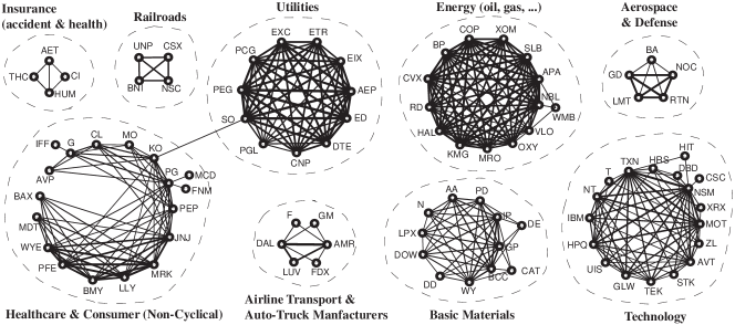
Figure 7: The stock network with the threshold $p_{c}=0.1$. The thickness of links indicates the strength of the correlation in the group correlation matrix.

We determine $p_{c}$ by observing the change of the network structure as $p$ decreases. Figure 6(a) displays the number of isolated clusters in the network as a function of threshold $p$. As we decrease $p$, the number of isolated clusters in the network increases slowly and stays near the maximum value up to $p=0.1$, and then it abruptly decreases to $1$, which indicates there exists only one isolated cluster. Therefore we choose $p_{c}=0.1$ to construct the most clustered but stable stock network comment3 .

We find that the constructed network consists of separable groups of stocks which correspond to the industrial sectors of stocks (see Fig. 7). At $p_{c}=0.1$, the network has $92$ nodes and $357$ links. The identification of stock group is very clear because the clusters in the network, which we consider to be equivalent to stock groups, are fully connected networks or very dense networks in which most of the nodes in the cluster are directly connected. However, although most of the stock groups are represented by a single industrial sector, it is found that the stocks which belong to two different industrial sectors coexist in a cluster. For instance, the stocks in the healthcare sector and the noncyclical consumer sector cannot be separable in this network. Indeed, in Fig. 5, one can observe non-negligible correlation between the healthcare and the noncyclical consumer, which indicates the presence of an intergroup correlation. In the real market, this presence of such an intersector correlation can be expected and our clustering results shown in Figs. 5 and 7 present both of intergroup and intragroup correlations that exist in the real stock market.

The group identification based on the eigenvector analysis of the stock price correlation matrix has been studied by several research groups Plerou2 ; Gopikrishnan ; Utsugi . In spite of their pioneering achievements to reveal the localization properties of eigenvectors, the classification of stocks into groups was not so clear, and it only covered about $10\%$ of their stocks because they used only the few highest contributions of eigenvector components due to the ambiguity explained in Sec. I. In this work, we not only introduce a more refined and systematic method to identify the stock groups, but also successfully cluster about $70\%$ of stocks into groups although direct comparison of the success ratio might be inappropriate because our data set is different from theirs.

On the other hand, Onnela et al. Onnela2 introduced the percolation approach to construct the stock network in which the links are added between stocks one by one in descending order from the highest element of the full correlation matrix. In their work, though highly correlated groups of stocks were found, the threshold value of the correlation to settle the network structure was hardly determined; the number of isolated clusters according to the threshold did not show the clear cut. We believe that this is attributed to the fact that they used the full correlation matrix carrying marketwide and random fluctuation. We would also fail to determine the critical threshold value of correlation if we use the full correlation matrix instead of the filtered one [see Fig. 6(b)]. This indicates that the filtering is crucial for the stock group identification.

Finally, we note that Marsili et al. introduced a different method to filter noises from the time series of stock price log-returns for stock group identification. In their work, it was assumed that the normalized log-return could be expressed by the linear combination of the noise at individual stock level and the noise at the level of the groups, which fitted to the real data to determine the weights of two noises and the constituents of the groups. However, we found that the effect of the inhomogeneous marketwide fluctuation is quite significant that the marketwide effect needs to be considered seriously to describe the correlation between stock correctly. Indeed, it is found that the filtering out of the corresponding $\mathrm{C}^{m}$ improves the clustering result.

IV Conclusion

In conclusion, we successfully identify the multiple group of stocks from the empirical correlation matrix of stock price changes in the New York Stock Exchange. We propose refined methods to find stock groups which dramatically reduce ambiguities as compared to identifying stock groups from the localization in a single eigenvector of the correlation matrix Plerou2 ; Gopikrishnan ; Utsugi . From the analysis of the characteristics of eigenvectors, we construct the group correlation matrix of the stock groups excluding the marketwide effect and random noise. By optimizing the representation of the group correlation matrix, we find that the group correlation matrix is represented by the block diagonal matrix where the stocks in each block belong to the same group. This coincides with the theoretical model of Noh Noh . Equally good stock group identification is also achieved by the percolation approach on the group correlation matrix to construct the network of stocks.

- (1) R. N. Mantegna and H. E. Stanley, An Introduction to Econophysics: Correlation and Complexity in Finance (Cambridge University Press, Cambridge, England, 2000); J. P. Bouchaud and M. Potters, Theory of Financial Rick (Cambridge University Press, Cambridge, England, 2000).
- (2) R. N. Mantegna, Eur. Phys. J. B 11, 193 (1999).
- (3) G. Bonanno, N. Vandewalle, and R. N. Mantegna, Phys. Rev. E 62, R7615 (2000).
- (4) G. Bonanno, G. Caldarelli, F. Lillo, and R. N. Mantegna, Phys. Rev. E 68, 046130 (2003).
- (5) J.-P. Onnela, A. Chakraborti, K. Kaski, J. Kertész, and A. Kanto, Phys. Rev. E 68 056110 (2003).
- (6) J.-P. Onnela, K. Kaski, and J. Kertész, Eur. Phys. J. B 38, 353 (2004).
- (7) L. Laloux, P. Cizeau, J.-P. Bouchaud, and M. Potters, Phys. Rev. Lett. 83, 1467 (1999)
- (8) V. Plerou, P. Gopikrishnan, B. Rosenow, L. A. Nunes Amaral, and H. E. Stanley, Phys. Rev. Lett. 83, 1471 (1999).
- (9) V. Plerou, P. Gopikrishnan, B. Rosenow, L. A. Nunes Amaral, T. Guhr, and H. E. Stanley, Phys. Rev. E 65, 066126 (2002).
- (10) P. Gopikrishnan, B. Rosenow, V. Plerou, and H. E. Stanley, Phys. Rev. E 64, 035106(R) (2001).
- (11) A. Utsugi, K. Ino, and M. Oshikawa, Phys. Rev. E 70, 026110 (2004).
- (12) L. Giada and M. Marsili, Phys. Rev. E 63, 061101 (2001); M. Marsili, Quant. Finance 2, 297 (2002); L. Giada and M. Marsili, Physica A 315, 650 (2002).
- (13) A. M. Sengupta and P.P. Mitra, Phys. Rev. E. 60, 3389 (1999).
- (14) Our selection of stocks covers most available stock price data for the period in the database. We use the adjusted daily stock prices and skip days of the data when splits and the dividends of any stock occur in Eqs. (1) and (2) to avoid the possible artifact caused by the abrupt stock price changes [see http://help.yahoo.com/help/us/fin/quote/index.html].
- (15) Z. Burda and J. Jurkiewicz, Physica A 344, 67 (2004).
- (16) P. Holme, M. Huss, and H. Jeong, Bioinformatics 19, 532 (2003).
- (17) J. D. Noh, Phys. Rev. E 61, 5981 (2000).
- (18) The similar matrix element rearranging technique was used in Ref. Bilke .
- (19) S. Bilke, e-print physics/0006050.
- (20) The visualization of is not very sensitive to the cutoff value .
- (21) S. Kirkpatrick, C. D. Gerlatt, and M. P. Vecchi, Science 220, 671 (1983).
- (22) W. H. Press, S. A. Teukolsky, W. T. Vetterling, and B. P. Flannery, Numerical Recipes in C (Cambridge University Press, Cambridge, England, 1992).
- (23) S.-W. Son, H. Jeong, and J. D. Noh, e-print cond-mat/0502672.
- (24) Small change of , , does not seriously change the clustering result.