Stabilization of three–dimensional light bullets by a transverse lattice in a Kerr medium with dispersion management

Abstract

We demonstrate a possibility to stabilize three–dimensional spatiotemporal solitons (“light bullets”) in self–focusing Kerr media by means of a combination of dispersion management in the longitudinal direction (with the group–velocity dispersion alternating between positive and negative values) and periodic modulation of the refractive index in one transverse direction, out of the two. The analysis is based on the variational approximation (results of direct three-dimensional simulations will be reported in a follow-up work). A predicted stability area is identified in the model’s parameter space. It features a minimum of the necessary strength of the transverse modulation of the refractive index, and finite minimum and maximum values of the soliton’s energy. The former feature is also explained analytically.

, , ,

1 Introduction

Search for spatiotemporal solitons in diverse optical media, alias “light bullets” (LBs) [1], is a challenge to fundamental and applied research in nonlinear optics, see original works [2, 3, 4, 5, 6, 7, 8, 9, 10] and a very recent review [11]. Stationary solutions for LBs can easily be found in the cubic ($\chi^{(3)}$) multi-dimensional nonlinear Schrödinger (NLS) equation [1], but their stability is a problem, as they are unstable against spatiotemporal collapse [12]. The problem may be avoided by resorting to milder nonlinearities, such as saturable [9], cubic-quintic [13], or quadratic ($\chi^{(2)}$) [2, 3, 4, 5, 6, 7, 8].

Despite considerable progress in theoretical studies, three-dimensional (3D) LBs in a bulk medium have not yet been observed in an experiment. The only successful experimental finding reported thus far was a stable quasi-2D spatiotemporal soliton in $\chi^{(2)}$ crystals [7] (the tilted-wavefront technique [14], used in that work, precluded achieving self-confinement in one transverse direction). On the other hand, it was predicted [8] that a spatial cylindrical soliton may be stabilized in a bulk medium composed of layers with alternating signs of the Kerr coefficient. Similar stabilization was then predicted for what may be regarded as 2D solitons in Bose-Einstein condensates (BECs), with the coefficient in front of the cubic nonlinear term subjected to periodic modulation in time via the Feshbach resonance in external ac magnetic field [15, 16]. However, no stable 3D soliton could be found in either realization (optical or BEC) of this setting.

Serious difficulties encountered in the experimental search for LBs in 3D media is an incentive to look for alternative settings admitting stable 3D optical solitons. With the Kerr nonlinearity, a possibility is to use a layered structure that periodically reverses the sign of the local group-velocity dispersion (GVD), without affecting the $\chi^{(3)}$ coefficient. This resembles a well-known scheme in fiber optics, known as dispersion management (DM), see, e.g., Refs. [17] and review [18]. A 2D generalization of the DM scheme was recently proposed, assuming a layered planar waveguide of this type, uniform in the transverse direction [19, 20]. As a result, large stability regions for the 2D spatiotemporal solitons were identified, including double-peaked breathers; however, a 3D version of the same model could not give rise to any stable soliton [19]. It was also shown in Ref. [19] that no stable 3D soliton could be found in a more sophisticated model, which combines the DM and periodic modulation of the Kerr coefficient in the longitudinal direction.

Another approach to the stabilization of multidimensional solitons was developed in the context of the self-attracting BEC. It is based on the corresponding Gross-Pitaevskii equation which includes a periodic potential created as an optical lattice (OL, i.e., an interference pattern produced by illuminating the condensate by counter-propagating coherent laser beams). It has been demonstrated that 2D [21, 22, 23] and 3D [21] solitons can be easily stabilized by the OL of the same dimension. Moreover, stable solitons can also be readily supported by low-dimensional OLs, i.e., 1D and 2D ones in the 2D [23, 24] and 3D [23, 24, 25] cases, respectively; additionally, a 3D soliton can be stabilized by a cylindrical (Bessel) lattice [26], similar to one introduced, in the context of 2D models, in Ref. [27]. On the other hand, 3D solitons cannot be stabilized by a 1D periodic potential [24]; however, the 1D lattice potential in combination with the above-mentioned time-periodic modulation of the nonlinearity, provided by the Feshbach resonance in the ac magnetic field, supports single- and multi-peaked stable 3D solitons in vast areas of the respective parameter space [28].

The above results suggest a possibility of existence of stable 3D “bullets” in a $\chi^{(3)}$ medium with the DM in the longitudinal direction ($z$), additionally equipped with an effective lattice potential (i.e., periodic modulation of the refractive index) in one transverse direction ($y$), while in the remaining transverse direction ($x$) the medium remains uniform. If this is possible, stable LBs will be definitely possible too in a medium with the periodic modulation of the refractive index in both transverse directions; however, the setting with one uniform direction is more interesting in terms of steering solitons and studying collisions between them [23, 24]. The objective of the present work is to predict such 3D spatiotemporal solitons and investigate their stability. Our first consideration of this possibility is based on the variational approximation (VA); systematic simulations of the 3D model are quite complicated, and will be presented in a follow-up work. It is relevant to mention that the existence and stability of 3D solitons in the Gross-Pitaevskii equation with the quasi-2D periodic potential, which were originally predicted by the VA[23, 24], was definitely confirmed by direct simulations [23, 24, 25], which suggests that in the present model the 3D solitons may easily be stable too.

The model is based on the normalized NLS equation describing the evolution of the local amplitude $u$ of the electromagnetic wave, which is a straightforward extension of the 2D model put forward in Ref. [19]:

$$i\frac{\partial u}{\partial z}+\left[\frac{1}{2}\left(\frac{\partial^{2}}{\partial x^{2}}+\frac{\partial^{2}}{\partial y^{2}}+D(z)\frac{\partial^{2}}{\partial\tau^{2}}\right)+\varepsilon\cos(2y)+|u|^{2}\right]u=0.$$ (1)

Here, $\varepsilon$ is the strength of the transverse modulation (the modulation period is normalized to be $\pi$), while $\tau$ and $D(z)$ are the same reduced temporal variable and local GVD coefficient as in the fiber-optic DM models [17, 18].

Equation (1) implies the propagation of a linearly polarized wave, with the single component $u$; a more general situation will be described by a two-component (vectorial) version of Eq. (1), with the two polarization coupled, as usual, by the cubic cross-phase-modulation terms. We do not expect that the vectorial model will produce results qualitatively different form those presented below. As usual, the NLS equation assumes the applicability of the paraxial approximation, i.e., the spatial size of solitons (see below) must be much larger than the underlying wavelength of light, which is definitely a physically relevant assumption [11], and the temporal part of the equation implies that the higher-order GVD is negligible (previous considerations have demonstrated that the higher-order dispersion does not drastically alter DM solitons [29]).

As is commonly adopted, we assume a symmetric DM map, with equal lengths $L$ of the normal- and anomalous-GVD segments (usually, the results are not sensitive to the map’s asymmetry),

$$D(z)=\left\{\begin{array}[]{l}\overline{D}+D_{\mathrm{m}}>0,\,0<z<L,\\ \overline{D}-D_{\mathrm{m}}<0,\,L<z<2L,\end{array}\right.$$ (2)

the average dispersion being much smaller than the modulation amplitude, $\left|\overline{D}\right|\ll D_{\mathrm{m}}$. Using the scaling invariances of Eq. (1), we fix $L\equiv 1$ and $D_{\mathrm{m}}\equiv 1$.

Recently, a somewhat similar 2D model was introduced in Ref. [30]. The most important difference is that it has the variable coefficient $D(z)$ multiplying both the GVD and diffraction terms, $u_{\tau\tau}$ and $u_{xx}$. Actually, that model was motivated by a continuum limit of some discrete systems; in the present context, it would be quite difficult to implement the periodic reversal of the sign of the transverse diffraction.

2 The variational approximation

Aiming to apply the VA for the search of LB solutions (a review of the variational method can be found in Ref. [18]), we adopt the Gaussian ansatz,

$$u = A(z)\exp\left\{\mathrm{i}\phi(z)-\frac{1}{2}\left[\frac{x^{2}}{W^{2}(z)}+\frac{y^{2}}{V^{2}(z)}+\frac{\tau^{2}}{T^{2}(z)}\right]\right.+$$ (3)

$$+\left.\frac{\mathrm{i}}{2}\left[b(z)\,x^{2}+c(z)\,y^{2}+\beta(z)\,\tau^{2}\right]\right\},$$

where $A$ and $\phi$ are the amplitude and phase of the soliton, $T$ and $W,V$ are its temporal and two transverse spatial widths, and $\beta$ and $b,c$ are the temporal and two spatial chirps. The Lagrangian from which Eq. (1) can be derived is

$$L = \frac{1}{2}\int_{-\infty}^{+\infty}\,\mathrm{d}x\int_{-\infty}^{+\infty}\,\mathrm{d}y\int_{-\infty}^{+\infty}\,\mathrm{d}\tau\left[\mathrm{i}\left(u_{z}u^{\ast}-u_{z}^{\ast}u\right)-\left|u_{x}\right|^{2}-\left|u_{y}\right|^{2}-D\left|u_{\tau}\right|^{2}\right.$$ (5)

$$\left.+2\varepsilon\cos(2y)|u|^{2}+|u|^{4}\right].$$

The substitution of the ansatz (3) in this expression and integrations lead to an effective Lagrangian, with the prime standing for $d/dz$:

$$(4/\pi^{3/2})L_{\mathrm{eff}} = A^{2}WVT\left[4\phi^{\prime}-b^{\prime}W^{2}-c^{\prime}V^{2}-\beta^{\prime}T^{2}-W^{-2}-V^{-2}-DT^{-2}\right.$$ (6)

$$\left.-b^{2}W^{2}-c^{2}V^{2}+\varepsilon\exp\left(-V^{2}\right)-D(z)\beta^{2}T^{2}+A^{2}/\sqrt{2}\right],$$

The first variational equation, $\delta L_{\mathrm{eff}}/\delta\phi=0$, applied to Eq. (6) yields the energy conservation, $dE/dz=0$, with

$$E\equiv A^{2}WVT.$$ (7)

The conservation of $E$ is used to eliminate $A^{2}$ from the set of subsequent equations, $\delta L_{\mathrm{eff}}/\delta\left(W,V,T,b,c,\beta\right)=0$. They can be arranged so as, first, to eliminate the chirps,

$$b=W^{\prime}/W,\,c=V^{\prime}/V,\beta=D^{-1}T^{\prime}/T.$$ (8)

the remaining equations for the spatial and temporal widths being

$$W^{\prime\prime} = \frac{1}{W^{3}}-\frac{E}{2\sqrt{2}W^{2}VT},$$ (9)

$$V^{\prime\prime} = \frac{1}{V^{3}}-4\varepsilon V\exp\left(-V^{2}\right)-\frac{E}{2\sqrt{2}WV^{2}T},$$ (10)

$$\left(\frac{T^{\prime}}{D}\right)^{\prime} = \frac{D}{T^{3}}-\frac{E}{2\sqrt{2}WVT^{2}}.$$ (11)

The Hamiltonian of these equations, which is a dynamical invariant in the case of constant $D$, is

$${\mathcal{H}}=\left(W^{\prime}\right)^{2}+\left(V^{\prime}\right)^{2}+\frac{\left(T^{\prime}\right)^{2}}{D}+\frac{1}{W^{2}}+\frac{1}{V^{2}}+\frac{D}{T^{2}}-4\varepsilon\exp(-V^{2})-\frac{E}{\sqrt{2}WVT}$$

In the case of the piece-wise constant modulation, such as in (2), the variables $W$, $W^{\prime}$, $V$, $V^{\prime}$, $T$ and $\beta$ must be continuous at junctions between the segments with $D_{\pm}\equiv\overline{D}\pm D_{\mathrm{m}}$. As it follows from Eq. (8), the continuity of the temporal chirp $\beta(z)$ implies a jump of the derivative $T^{\prime}$ when passing from $D_{-}$ to $D_{+}$, or vice versa:

$$\left(T^{\prime}\right)_{D=D_{+}}=\left(D_{+}/D_{-}\right)\left(T^{\prime}\right)_{D=D_{-}}.$$ (12)

In the case of a continuous DM map, rather than the one (2), Eq. (11) has a formal singularity at the points where $D(z)$ vanishes, changing its sign. However, it is known that there is no real singularity in this case, as $T^{\prime}$ vanishes at the same points, which cancels the singularity out [18].

In the absence of the DM and transverse modulation, i.e., $D\equiv+1$ and $\varepsilon=0$, three equations (9) - (11) reduce to one, which is tantamount to the variational equation derived in Ref. [31] from the spatiotemporally isotropic ansatz [cf. Eq. (3)], $u=A\exp\left[\mathrm{i}\phi-(1/2)\left(W^{-2}+\mathrm{i}b\right)\left(x^{2}+y^{2}+\tau^{2}\right)\right]$. In particular, this single equation correctly predicts the asymptotic law of the strong collapse in the 3D case, which is stable against anisotropic perturbations [32], $V=W=T\approx\left(5E/3\sqrt{2}\right)^{1/5}\left(z_{0}-z\right)^{2/5}$, $z=z_{0}$ being the collapse point. The location of this point is determined by initial conditions, but, in any case, it belongs to an interval $D>0$, where the GVD is anomalous.

Another possible collapse scenario is an effectively two-dimensional (weak) one, with two widths shrinking to zero as $z_{0}-z\rightarrow 0$, while the third one remains finite. For instance, the corresponding asymptotic law may be

$$V=T=A\left(z_{0}-z\right)^{1/2},~{}W=\frac{\sqrt{2}E}{4+A^{4}}-\frac{\left(4+A^{4}\right)^{2}}{4\sqrt{2}EA^{2}}\left(z_{0}-z\right)\ln\left(z_{0}-z\right),$$ (13)

where $A$ is a positive constant or else $V=2/T\sim(z_{0}-z)^{1/2}$ and $W\rightarrow W_{0}$ (in this case too, the collapse point $z_{0}$ must belong to a segment with $D>0$). In direct simulations of Eqs. (9) - (11), we actually observed only the latter scenario. However, we did not specially try to find initial conditions that could initiate a solution corresponding to the strong 3D collapse, as our objective is not the study of the collapse, but rather search for solitons stable against collapse. In fact, known results for the solitons in the 3D Gross-Pitaevskii equation with the OL potential suggest that, while the VA may be incorrect in the description of the collapse, as a singular solution, it provides for quite accurate predictions for the stability of solitons as regular solutions [23, 24].

If the DM is absent, and the constant GVD is normal, i.e., $D\equiv-1$, only the 2D collapse in the transverse plane would be possible, so that (cf. Eq. (13))

$$V=W=A\left(z_{0}-z\right)^{1/2},~{}T=\frac{\sqrt{2}E}{4+A^{4}}+\frac{\left(4+A^{4}\right)^{2}}{4\sqrt{2}EA^{2}}\left(z_{0}-z\right)\ln\left(z_{0}-z\right).$$

However, we did not observed this collapse scenario in our simulations. The same comment as one given above pertains to this case as well.

A possibility of the stabilization of the 3D soliton by a sufficiently strong lattice can be understood noticing that, for large $\varepsilon$, one may keep only the first two terms on the right-hand side of Eq. (10). This approximation yields a nearly constant value $V_{0}$ of $V$, which is a smaller root of the corresponding equation,

$$4\varepsilon V_{0}^{4}\exp\left(-V_{0}^{2}\right)=1$$ (14)

(a larger root corresponds to an unstable equilibrium). The two roots exist provided that

$$\varepsilon>\varepsilon_{\mathrm{\min}}=\mathrm{e}^{2}/16\approx\allowbreak 0.46,$$ (15)

the relevant one being limited by $V_{0}<2$. Then, the substitution of $V=V_{0}$ in the remaining equations (9) and (11) leads to essentially the same VA-generated dynamical system as derived for the 2D DM model in Ref. [19], which was shown to give rise to stable spatiotemporal solitons. On the other hand, it was demonstrated in Ref. [19] too that, in the case of $\varepsilon=0$, the 3D VA equations, as well as the full underlying 3D model, have no stable soliton solutions.

The stabilization of the LB in the present model for large $\varepsilon$ can also be understood in a different way, without resorting to VA: in a very strong lattice, the soliton is trapped entirely in a single “valley” of the periodic potential, and the problem thus reduces to a nearly 2D one, where spatiotemporal solitons may be stable, cf. a similar stabilization mechanism for the solitons in the Gross-Pitaevskii equations developed in [16]. From this point of view, a really interesting issue is to find an actual minimum $\varepsilon_{\min}$ of the lattice’s strength which is necessary for the stabilization of the 3D solitons, as at $\varepsilon$ close enough to $\varepsilon_{\mathrm{\min}}$ the stabilized solitons are truly 3D objects, rather than their nearly-2D counterparts.

3 Results

We explored the parameter space of the variational system (9) - (11), $\left(E,\varepsilon,\overline{D}\right)$, by means of direct simulations of the equations (with regard to the jump condition (12)). As a result, it was possible to identify regions where the model admits stable solitons featuring regular oscillations in $z$ with the DM-map period. An example of such a regime is shown in Fig. 1 (oscillations in the evolution of $W$ are not visible in the figure because, as an estimate demonstrates, their amplitude is $\simeq 0.001$).

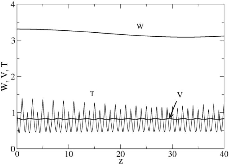
Figure 1: An example of the stable evolution of solutions to the variational equations (9) - (11). The soliton’s widths in the direction $x,y$ and $\tau$, i.e., $W,V$ and $T$, are shown as functions of $z$, for $E=0.5$, $\varepsilon=1$, and $\overline{D}=0$.

Systematic results obtained from the simulations are summarized in stability diagrams displayed in Figs. 2 and 3. A remarkable fact, apparent in Fig. 2, is that the minimum value of the lattice’s strength, $\varepsilon_{\min}=0.46$, at which the solitons may be stable, coincides with the analytical prediction (15), up to the available numerical accuracy.

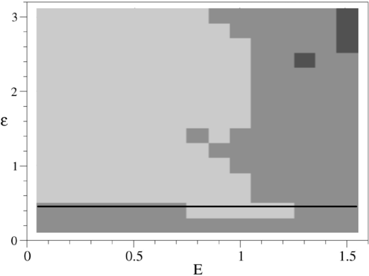
Figure 2: The stability area for the 3D spatiotemporal solitons in the $\left(E,\varepsilon\right)$ plane, with $\overline{D}=0$, is shown by light-gray shading. In gray and dark-gray regions, the 3D soliton is predicted, respectively, to spread out and collapse. The vertical line corresponds to the analytically predicted threshold (15).

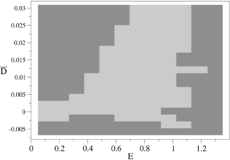
Figure 3: The stability area in the $\left(E,\overline{D}\right)$ plane, with $\varepsilon=1$, is shown by light–gray shading. In the gray region, the 3D soliton is predicted to spread out.

The existence of a maximum value $E_{\max}$ of the energy admitting the stable LBs is, essentially, a quasi-2D feature, which can be understood assuming that the potential lattice is strong. Indeed, as explained above, in such a case the value of $V$ is approximately fixed as the smaller root of Eq. (14). Within a segment where the GVD coefficient keeps the constant value, $D_{+}=\overline{D}+D_{\mathrm{m}}>0$, which corresponds to anomalous dispersion (see Eq. (2), the remaining equations (9) and (11) are tantamount to those for a uniform 2D Kerr-self-focusing medium, hence the energy is limited by the value $E_{\max}$ corresponding to the Townes soliton; the soliton will collapse if $E>E_{\max}$ [12].

The fact that the region of stable solitons is also limited by a minimum energy, $E_{\min}$, except for the case of $\overline{D}=0$, when $E_{\min}=0$ (see Fig. 3)), is actually a quasi-1D feature, which is characteristic to the DM solitons in optical fibers. In that case, the term $\sim E$ in the evolution equation for $T(z)$, cf. Eq. (11), is necessary to balance the average GVD coefficient $\overline{D}$, so that $E_{\min}$ and $\overline{D}$ vanish simultaneously [17]. It is noteworthy too that, as well as in the case of the 1D DM solitons in fibers, the stability area in Fig. 3 includes a part with normal average GVD, $\overline{D}<0$, which seems counterintuitive, but can be explained [17]. This part extends in Fig. 3 up to $\left(-\overline{D}\right)_{\max}\approx 0.005$.

4 Conclusions

In this work, we have proposed a possibility to stabilize spatiotemporal solitons (“light bullets”) in three-dimensional self-focusing Kerr media by means of the dispersion management (DM), which means that the local group-velocity dispersion coefficient alternates between positive and negative values along the propagation direction, $z$. Recently, it was shown that the DM alone can stabilize solitons in 2D (planar) waveguides, but in the bulk (3D) DM medium the “bullets” are unstable. In this work, we have demonstrated that the complete stabilization can  be provided if the longitudinal DM is combined with periodic modulation of the refractive index in one transverse direction ($y$), out of the two. The analysis was based on the variational approximation (systematic results of direct simulations will be reported in a follow-up paper). A stability area for the light bullets was identified in the model’s parameter space. Its salient features are a necessary minimum strength of the transverse modulation of the refractive index, and minimum and maximum values $E_{\min,\max}$ of the soliton’s energy. The former feature can be accurately predicted (see Eq. (15)) in an analytical form from the evolution equation for the width of the soliton in the $y$-direction. The existence of $E_{\min}$, which vanishes when we assume zero average dispersion, can be explained in the same way as for the temporal solitons in DM optical fibers. Also, similar to the case of DM solitons in fibers, we find that the stability area extends to a region of normal average dispersion [17]. On the other hand, the existence of $E_{\max}$ can be understood similarly to as it was recently done in the 2D counterpart of the present model (the strong transverse lattice can squeeze the system to a nearly 2D shape).

The results presented in this work suggest a new approach to the challenging problem of the creation of 3D spatiotemporal optical solitons. The model also opens a way to address advanced issues, such as collisions between the LBs, and the existence and stability of solitons with different symmetries (for instance, LBs which are odd in the longitudinal and/or transverse directions). These issues will be considered elsewhere.

5 Acknowlegdements

M.M., M.T. and E.I. acknowledge support from KBN Grant No. 2P03 B4325. B.A.M. acknowledges the hospitality of the Physics Department and Soltan Institute for Nuclear Studies at the Warsaw University, and partial support from the Israel Science Foundation grant No. 8006/03. This author also appreciates the help of A. Desyatnikov in making Ref. [23] available on the internet.

References

- [1] Y. Silberberg, Opt. Lett. 15 (1990) 1282.
- [2] A.A. Kanashov and A.M. Rubenchik, Physica D 4 (1981) 122.
- [3] K. Hayata and M. Koshiba, Phys. Rev. Lett. 71 (1993) 3275.
- [4] B.A. Malomed, P. Drummond, H. He, A. Berntson, D. Anderson, M. Lisak, Phys. Rev. E 56 (1997) 4725; D. V. Skryabin and W. J. Firth, Opt. Commun. 148 (1998) 79; D. Mihalache, D. Mazilu, B.A. Malomed, L. Torner, Opt. Commun. 152 (1998) 365; D. Mihalache, D. Mazilu, J. Dörring, L. Torner, Opt. Commun. 159 (1999) 129.
- [5] M. Blaauboer, B.A. Malomed, G. Kurizki, Phys. Rev. Lett. 84 (2000) 106; M. Blaauboer, G. Kurizki, B.A. Malomed, Phys. Rev. E 62 (2000) R57.
- [6] L. Torner, S. Carrasco, J.P. Torres, L.-C. Crasovan, D. Mihalache, Opt. Commun. 199 (2001) 277.
- [7] X. Liu, L. J. Qian, F. W. Wise, Phys. Rev. Lett. 82 (1999) 4631; X. Liu, K. Beckwitt, F. Wise, Phys. Rev. E 62 (2000) 1328.
- [8] I. Towers and B.A. Malomed, J. Opt. Soc. Am. 19 (2002) 537.
- [9] D. E. Edmundson, R. H. Enns, Opt. Lett. 17 (1992) 586; R. H. Enns, R. H., S. S. Rangnekar, Phys. Rev. A 45 (1992) 3354; R. H. Enns, D. E. Edmundson, S. S. Rangnekar, A. E. Kaplan, Opt. Quant. Electr. 24 (1992) S1295.
- [10] R. McLeod, K. Wagner and S. Blair, Phys. Rev. A 52 (1995) 3254.
- [11] B. A. Malomed, D. Mihalache, F. Wise, L. Torner, Spatiotemporal optical solitons, J. Opt. B: Quant. Semicl. Opt., in press.
- [12] L. Bergé, Phys. Rep. 303 (1998) 260.
- [13] A. Desyatnikov, A. Maimistov, B. Malomed, Phys. Rev. E 61 (2000) 3107; D. Mihalache, D. Mazilu, L.-C. Crasovan, I. Towers, A. V. Buryak, B. A. Malomed, L. Torner, J. P. Torres, F. Lederer, Phys. Rev. Lett. 88 (2002) 073902.
- [14] P. Di Trapani, D. Caironi, G. Valiulis, A. Dubietis, R. Danielius, A. Piskarskas, Phys. Rev. Lett. 81 (1998) 570.
- [15] H. Saito and M. Ueda, Phys. Rev. Lett. 90 (2003) 040403; F. Kh. Abdullaev, J. G. Caputo, R. A. Kraenkel, B.A. Malomed, Phys. Rev. A 67 (2003) 013605.
- [16] G. D. Montesinos, V. M. Pérez-García, P. J. Torres, Physica D 191 (2004) 193.
- [17] J. H. B. Nijhof, N. J. Doran, W. Forysiak and F. M. Knox, Electron. Lett. 33 (1997) 1726; T. Lakoba, J. Yang, D. J. Kaup, B. A. Malomed, Optics Commun. 149 (1998) 366; S. K. Turitsyn and E. G. Shapiro, Opt. Lett. 23 (1998) 682; J. N. Kutz and S. G. Evangelides, Opt. Lett. 23 (1998) 685.
- [18] B. A. Malomed, Progr. Optics 43 (2002) 69.
- [19] M. Matuszewski, M. Trippenbach, B. A. Malomed, E. Infeld, A. A. Skorupski, Phys. Rev. E 70 (2004) 016603.
- [20] M. I. Rodas-Verde, G. D. Montesinos, H. Michinel, V. M. Pérez-García, nlin/0407037.
- [21] B. B. Baizakov, B. A. Malomed, M. Salerno, Europhys. Lett. 63 (2003) 642.
- [22] J. Yang and Z. H. Musslimani, Opt. Lett. 28 (2003) 2094.
- [23] B. B. Baizakov, M. Salerno, B. A. Malomed, in: Nonlinear Waves: Classical and Quantum Aspects, ed. by F. Kh. Abdullaev and V. V. Konotop, p. 61 (Kluwer Academic Publishers: Dordrecht, 2004); also available at http://rsphy2.anu.edu.au/~asd124/Baizakov_2004_61_NonlinearWaves.pdf
- [24] B. B. Baizakov, B. A. Malomed, M. Salerno, Phys. Rev. A 70 (2003) 053613.
- [25] D. Mihalache, D. Mazilu, F. Lederer, Y. V. Kartashov, L.-C. Crasovan, L. Torner, Phys. Rev. E 70 (2004) 055603(R).
- [26] D. Mihalache, D. Mazilu, F. Lederer, B. A. Malomed, Y. V. Kartashov, L.-C. Crasovan, L. Torner, Stable spatiotemporal solitons in Bessel optical lattices, to be published.
- [27] Y. V. Kartashov, V. A. Vysloukh, L. Torner, Phys. Rev. Lett. 93 (2004) 093904.
- [28] M. Trippenbach, M. Matuszewski, B. A. Malomed, Stabilization of three-dimensional matter-waves solitons in an optical lattice, Europhys. Lett., in press.
- [29] D. Frantzeskakis, K. Hizanidis, B.A. Malomed, H. E. Nistazakis, Pure Appl. Opt. 7 (1998) L57; T. I. Lakoba and G. P. Agrawal, J. Opt. Soc. Am. B 16 (1999) 1332.
- [30] F. Kh. Abdullaev, B. B. Baizakov, M. Salerno, Phys. Rev. E 68 (2003) 066605.
- [31] M. Desaix, D. Anderson, M. Lisak, J. Opt. Soc. Am. B 8 (1991) 2082.
- [32] S. N. Vlasov, L. V. Piskunova, V. I. Talanov, Sov. Phys. JETP 68 (1989) 1125.