Recurrence time analysis, long-term correlations, and extreme events

Abstract

The recurrence times between extreme events have been the central point of statistical analyses in many different areas of science. Simultaneously, the Poincaré recurrence time has been extensively used to characterize nonlinear dynamical systems. We compare the main properties of these statistical methods pointing out their consequences for the recurrence analysis performed in time series. In particular, we analyze the dependence of the mean recurrence time and of the recurrence time statistics on the probability density function, on the interval whereto the recurrences are observed, and on the temporal correlations of time series. In the case of long-term correlations, we verify the validity of the stretched exponential distribution, which is uniquely defined by the exponent $\gamma$, at the same time showing that it is restricted to the class of linear long-term correlated processes. Simple transformations are able to modify the correlations of time series leading to stretched exponentials recurrence time statistics with different $\gamma$, which shows a lack of invariance under the change of observables.

I Introduction

Recurrence time analysis is a powerful tool to characterize temporal properties of well defined events bunde ; bunde.prl . It has been recently extensively performed in a rich variety of experimental time series: records of the climate bunde2 ; santhanam ; alley , seismic activities earthquakes , solar flares boffetta.prl , spikes in neurons joern , turbulence in magnetic confined plasma murilo.plasma and stock market indices murilo.bolsa . Calculated essentially in the same way, these analyses receive different names: waiting time distribution, interocurrence time statistics, distribution of interspike intervals, distribution of laminar phases, etc. Through a unified perspective, we discuss the main properties of these statistical methods, which allows us to reinterpret and specify many previous results. By a careful discussion of the relevance of the probability density function (PDF) of the time series data we can easily understand and, in a particular case, reject results on earthquake statistics (Sec. II). In the case of long-term correlated linear time series we obtain a closed expression for the stretched exponential distribution of recurrence times which is valid for different recurrence intervals. We show also the lack of invariance of the long-term correlations of the time series under transformations that simulate the choice of different observables of the system (Sec. III). Before reporting these results we start with a proper definition of time series recurrence times, we compare it to the Poincaré recurrences and we discuss briefly some important recent applications of the recurrence time analysis.

I.1 Recurrence times

Time series recurrences
Assuming a time series point of view, in this paper we study the statistical properties of the recurrence time $T$. Given a time series $\{x_{n}\},n=1,\ldots,N$, and having defined a recurrence interval $I$ as a subset of the data range, then the $i$th recurrence time $T_{i}$ is the time interval $\Delta n$ between the $i$th and the $i+1$st visit of a time series point in $I$. The recurrence time statistics (RTS) is obtained as the distribution $P(T)$ of the sequence of recurrence times $T_{i}$.

Evidently, the sequence of recurrence times generated this way depends sensitively on the choice of $I$, which in fact will be one prominent issue of this paper. While for the recurrence of extreme events the recurrence interval is defined by the points above a threshold bunde

$$I_{ext}(q)=[q,\infty[\;,$$ (1)

in a more general way it may be defined around a position $X_{c}$ with a semi-width $\delta$ murilo.plasma ; altmann

$$I(X_{c},\delta)=[X_{c}-\delta,X_{c}+\delta]\;.$$ (2)

Both kinds of intervals are illustrated in Fig. 1.

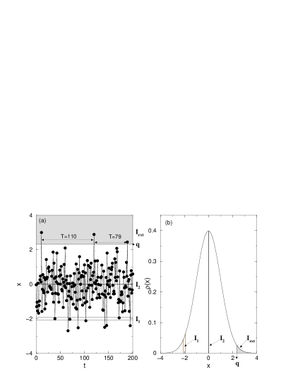
Figure 1: Gaussian distributed time series with recurrence intervals with measure $\mu(I)=0.01$, what implies $\langle T\rangle=100$. One extreme interval $I_{ext}(q=2.3263)=[2.3263,\infty[$ and two recurrence intervals $I_{1}(-2,0.0922)=[-1.9078,-2.0922]$, $I_{2}(0,0.0125)=[-0.0125,0.0125]$ illustrated in the (a) time series and (b) probability density function.

Poincaré recurrences
In dynamical systems’ theory, another concept of recurrence, known as Poincaré recurrences, plays a central role. Given a closed Hamiltonian system with ergodicity on the energy shell, the famous Poincaré recurrence theorem asserts that almost all trajectories (except for a set of zero measure) started inside some subset ${\cal V}$ of the phase space $\Gamma$ will return to it infinitely many times. In the limit of vanishing volume of this subset, the time between consecutive recurrences is the Poincaré recurrence time. Despite the well known debates about the foundations of statistical mechanics (Zermello paradox) these ideas motivated throughout the years also mathematical studies kac and, more recently, applications of recurrence analysis to many different dynamical systems (see Ref. zas.pr and references therein).

Surprisingly, as far as we know, no connection between the two recurrence approaches described above were made until now. The most evident way to establish this relationship is to define an observable $x=x(\vec{\gamma})$, when $\vec{\gamma}(t)\in\Gamma$ is the trajectory in phase space of the Hamiltonian system. The recurrence volume ${\cal V}$ is mapped to an interval $I_{\cal V}$ on the real axis by the observation function $x(\vec{\gamma})$. However, the sequence of recurrence times of the series $x_{n}:=x(\vec{\gamma}(t=n\Delta t))$ with respect to $I_{\cal V}$ is generally not identical to the sequence of Poincaré recurrences of $\vec{\gamma}(t)$ with respect of ${\cal V}$, since there is usually a large set $\bar{\cal V}$ which also maps to $I_{\cal V}$ due to the non-invertibility of $x(\vec{\gamma})$. Moreover, generally $I_{\cal V}$ will be of the kind of $I(X_{c},\delta)$ rather than $I_{ext}(q)$.

However, as we will show in this paper, the analogy with Poincaré recurrences motivates issues related to the recurrence times of extreme events which will reveal fundamental insight into their properties. Two main results will be the lack of invariance of the RTS under change of the observable and the fact that long-term correlations are not fully characterized by the autocorrelation function.

I.2 Earthquakes and SOC models

The recurrence time between extreme events was recently used in the analysis of different experimental time series bunde2 ; santhanam ; alley ; joern ; boffetta.prl ; earthquakes . One of the most important examples of this analysis, which is going to be discussed later in this paper, is the study of the waiting time between earthquakes or avalanches in models exhibiting self-organized criticality (SOC). The idea of studying recurrences in SOC started with the first connections between SOC and earthquakes sornette . More recently, the investigation of seismic catalogs of different regions of the globe indicate the existence of a universal distribution of recurrence times between big earthquakes earthquakes , which may be roughly described as a power-law distribution

$$P(T)\propto T^{-\alpha},$$ (3)

followed by a faster decay. Simple SOC models have a Poisson (exponential) distribution of recurrence times, what was used as argument against the use of SOC to model not only earthquakes yang.prl but also (and originally) solar flares boffetta.prl . However, non-Poissonian distributions are obtained in more sophisticated SOC models sanchez.prl ; christiansen , what keeps open the debate over the use of SOC in these fields, with the RTS as one of its central ingredients.

I.3 Long-term correlations and recurrence times

If time series data $\{x_{n}\}$ are exponentially (short range) correlated, the RTS is well known to be Poissonian, i.e., exponential for all $T$, independent of the choice of $I$ (in the limit of small interval $\mu(I)\rightarrow 0$) altmann . The same result applies to Poincaré recurrences (including independence of ${\cal V}$) if the underlying dynamics is hyperbolic, i.e., in well defined mathematical way fully chaotic hirata . Also in this case, correlations decay fast. Hence, for systems with an exponential decay of correlations, details of defining recurrence times and further details of the system are irrelevant; instead there exists a unique RTS.

Many time series data have been found to be long-term correlated, i.e., their mean autocorrelation time diverges bunde2 ; santhanam ; kantelhardt . Typically, this situation is characterized in the time series $\{x_{n}\}$ (assuming $\langle x_{n}\rangle=0$) by the exponent $0<\gamma_{c}<1$ of the power-law decay of the autocorrelation function as a function of the time $s$

$$C_{x}(s)=\langle x_{i}x_{i+s}\rangle=\frac{1}{N-s}\sum_{i=1}^{N-s}x_{i}x_{i+s}\sim s^{-\gamma_{c}}\;.$$ (4)

In a recent paper bunde , Bunde et al. analyzed the effect of long-term correlations on the return periods of extreme events, i.e., of recurrence times obtained using recurrence intervals of type (1). The main results of Ref. bunde ; bunde.prl for long-term correlated time series can be summarized by the following three points. While the first was obtained considering statistical arguments, the two others were based on numerical simulations.
(i) The mean recurrence time is equal to the inverse of the fraction of extreme points in the series

$$\langle T\rangle=\frac{N_{total}}{N_{extreme}}.$$

(ii) The statistics of $T$ follows a stretched exponential

$$\ln P(T)\propto-(T/\langle T\rangle)^{\gamma}\;,$$ (5)

where $\gamma=\gamma_{c}$ is identical to the correlation exponent in Eq. (4).
(iii) The series of recurrence times is long-term correlated with an exponent $\gamma_{T}$ close to $\gamma_{c}$.

Statement (i) is the time series analogous of Kac’s Lemma (Sec. II), statement (ii) will be verified carefully (Sec. III.2) once we have established the full functional form of the stretched exponential (5), and statement (iii) seems not to be generally valid (Sec. III.4).

Even if one might argue that based on Ref. bunde the validity of Eq. (5) is established only for the class of the model data chosen there, the reproduction of these findings for empirical data bunde2 ; santhanam suggests some generality of the stretched exponential distribution. Here, the link to Poincaré recurrences shows the opposite: Hamiltonian systems with mixed phase space are long-term correlated and show power-law tails in the statistics of Poincaré recurrence times zas.pr . In this case, the long-term correlations are originated by the stickiness of chaotic trajectories near the border of integrable islands. They cause a kind of intermittent dynamics and manifest themselves in complicated higher-order temporal correlations. In fact, the temporal properties of typical data are not fully specified by the autocorrelation function, Eq. (4), what explains why there cannot be a unique RTS for long-term correlated data. Connections between the long-term correlation exponent $\gamma_{c}$ and the RTS have to be established independently in every class of long-term correlated dynamical systems, as was done for Hamiltonian systems with mixed phase space zas.pr and fractal renewal point processes thurner . We argue in Sec. III.2 that the results of Ref. bunde described above are valid for long-term correlated linear time series bunde.prl . In this paper we propose a closed expression for the RTS of time series of this class, which is valid for recurrence intervals of both types (1) and (2).

II Mean recurrence time

The mean recurrence time

$$\langle T\rangle\equiv\lim_{N_{e}\rightarrow\infty}\frac{1}{N_{e}}\sum_{1}^{N_{e}}T_{i},$$

is a direct result of the choice of the recurrence interval. In area preserving dynamical systems Kac’s lemma kac states that the inverse of $\langle T\rangle$ is equal to the ergodic measure of the recurrence interval $\mu(I)$. In the case of stationary time series, as illustrated in Fig. 1, an equivalent result is obtained from the normalized PDF $\rho(x)$,

$$\frac{\Delta t}{\langle T\rangle}=\mu(I)\equiv\int_{x\in I}\rho(x)dx,$$ (6)

where $\Delta t$ is the sampling rate used to record the time series. This is the most important constraint to the statistics of recurrence times. In the time series analysis this measure is estimated as the fraction of valid events (points inside the recurrence interval) $\mu(I)=N_{events}/N$. Intuitively, relation (6) states simply that the total observation time $t$ is given by

$$t=N\Delta t=N_{events}\langle T\rangle.$$

Besides the RTS $P(T)$ the PDF $\rho(x)$ of the series of points itself is typically used to characterize the time series. Contrary to other time series analyses (as the detrended fluctuation analysis discussed below), the RTS is independent of the PDF. In particular, it is irrelevant whether the second moment of the PDF is finite. A time series with a well behaved (Gaussian) PDF can have either exponential or power-law RTS . Reversely, a time series with fat tails in the PDF can lead to a RTS that might be Poisson or power-law . The reason for this is simple: the RTS depends on the sequence of the time series points and changes under their temporal rearrangement, which does not change the PDF of the data. While the RTS is independent of the PDF of the series, the opposite happens to the mean recurrence time $\langle T\rangle$. Once the recurrence interval is defined, whether by relation (1), (2) or by any other possible definition, the PDF $\rho(x)$ provides $\langle T\rangle$ through relation (6).

These two apparently trivial observations, i.e., independence of the RTS and dependence of $\langle T\rangle$ on the PDF, shed new light on previous results. In what follows, we exemplify these points in the analysis of recurrence times between earthquakes, already mentioned in Sec. I.2. Despite (or because of) the complexity of this field it has an important simplicity: the Gutenberg-Richter law

$$\rho(M)\propto e^{-b\;\ln(10)M}\;,$$ (7)

where $A,b$ are constants and $M$ is the magnitude of the earthquake, which is proportional to the logarithm of the released energy. The constant $b$ is almost the same for different parts of the world and the empirical law (7) is valid for $2\leq M\lesssim 7.5$. From our perspective this means that the PDF of the time series of seismic activity is given.

The mean recurrence time between earthquakes of a given magnitude $M$ is obtained inserting the PDF given by (7) in relation (6), and using the interval of the type (2) with $X_{c}=M$,

$$\langle T\rangle(M)=T_{0}e^{b\;ln(10)M}\;,$$ (8)

where $T_{0}\propto\frac{b\;ln(10)}{(1-e^{-b\;ln(10)\delta})}$. This relation is equivalent to the one obtained previously through a “mean-field approach” sornette . In Ref. sanchez.prl it is noted the “remarkable” scaling of $\langle T\rangle(M\geq M_{c})\propto 10^{bM_{c}}$, which is nothing else than a consequence of relation (6) when intervals of the type (1) are used with $q=M_{c}$.

So far, the relation between $\langle T\rangle$ and the PDF was used to show that the mean waiting time between earthquakes is directly related to the Gutenberg-Richter law, but has nothing to do with temporal correlations between earthquakes. On the other hand, the RTS obtained from earthquakes records earthquakes is an independent result that can be used as a test for the dynamical models of earthquakes. Recently, it was suggested that in SOC models the sequence of avalanches is uncorrelated boffetta.prl ; yang.prl (see joern2 for a counterexample) and should thus be discarded. The solution of this debate is beyond the scope of this paper. Nevertheless, we note that, as a consequence of the unrelatedness of $\rho(x)$ and $P(T)$, shuffling data of whatever distribution randomly (as was done for the time series of seismic activity in Ref. yang.prl ) trivially implies $P(T)$ of being exponential, also for finite recurrence intervals altmann .

III Statistics of recurrence times

III.1 Closed expression of the stretched exponential distribution

We generalize the distribution proposed in Ref. bunde for the RTS of long-term correlated time series. Motivated by result (ii), mentioned in Sec. I.3, suppose that the stretched exponential distribution

$$P_{\gamma}(T)=ae^{-(bT)^{\gamma}}$$ (9)

is valid for all recurrence times $T\in~{}]0,\infty[$. This is actually a stronger assumption than Eq. (5). As any RTS, Eq. (9) must satisfy the following two conditions: normalization

$$\int_{0}^{\infty}P(T)dT=1,$$

and the analogous of Kac’s lemma (6)

$$\langle T\rangle\equiv\int_{0}^{\infty}TP(T)dT=\frac{1}{\mu(I)}.$$

Imposing these two conditions to the distribution (9), it is possible to express the constants $a$ and $b$ as functions of $\gamma$ and $\mu(I)$. Further simplification is obtained performing the following transformation of variables $\tau=\frac{T}{<T>}=\mu(I)T$, i.e., counting the time in units of the mean recurrence time. The complete stretched exponential distribution for recurrence times is then written as

$$p_{\gamma}(\tau)=a_{\gamma}e^{-(b_{\gamma}\;\tau)^{\gamma}},\mbox{ with}\left\{\begin{array}[]{ll}a_{\gamma}=&b_{\gamma}\;\frac{\gamma}{\Gamma(1/\gamma)},\\ \\ b_{\gamma}=&\frac{(2^{1/\gamma})^{2}\Gamma(\frac{2+\gamma}{2\gamma})}{2\sqrt{\pi}},\end{array}\right.$$ (10)

and depends exclusively on the exponent $\gamma$.

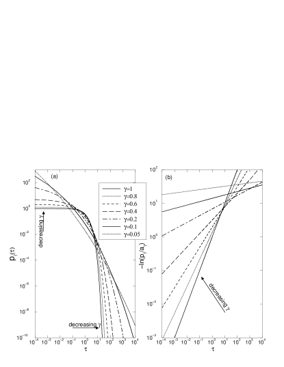
Figure 2: The stretched exponential distribution (10) for different values of the exponent $\gamma$.

Equation (10) is illustrated in Fig. 2 for different values of $\gamma$ in two different ways. Graph (a) (log-log) shows that decreasing the value of $\gamma$ the distribution starts from the exponential (Poisson) case ($\gamma=1$) and approaches a power-law ($\gamma\rightarrow 0$) with an exponent $\alpha=1.5$. Graph (b) shows the distribution in the form that the stretched exponentials are seen as straight lines bunde ; bunde2 ; santhanam . Generally, to obtain graph (b) from (a) one needs to divide the distribution $P(T)$ by the correct pre-factor $a=P(0)$, which is typically unknown. Distribution (10) shows the dependence of the pre-factor $a$ on the exponent $\gamma$ when the stretched exponential $p_{\gamma}(\tau)$ is valid in the whole interval of times. For experimental or numerical data, where neither $a$ nor $\gamma$ are known a priori, the relation between both is useful to correctly visualize and fit the RTS. We note that in practice the numerical fitting of the exponent $\gamma$ is very sensitive and typically depends on the choice of the pre-factor $a$.

III.2 Numerical results for long-term correlated linear time series

We compare now the stretched exponential distribution (10) to the numerical results of the RTS obtained in long-term correlated time series. As in Ref. bunde , the data were generated using the Fourier transform technique prakash : imposing a power-law decay on the Fourier spectrum

$$f_{x}(k)\propto k^{-\beta}\;,$$ (11)

with $0<\beta<0.5$ and choosing phase angles at random, we obtain through an inverse Fourier transform the long-term correlated time series in $x$ with $\gamma_{c}=1-2\beta$ in Eq. (4). The data are Gaussian distributed with $\langle x\rangle=0,\sigma=1$, and Eq. (6) was used to calculate the times $\tau=T/\langle T\rangle$.

Having specified the power spectrum or, correspondingly, the autocorrelation function for sequences of Gaussian random numbers means to have fixed all parameters of a linear stochastic process. Hence, in principle, the coefficients of an auto regressive (AR($r$)) or moving average (MA($r$)) process can be uniquely determined, where, due to the power-law nature of spectrum and autocorrelation function, the orders $r$ of either of these models have to be infinite box . Hence, the following results are valid for the class of linear long-term correlated processes bunde.prl . In other words, higher order correlations for this class of processes follow trivially from the two-point correlations.

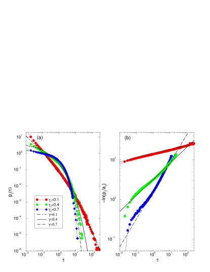
Figure 3: (color online) RTS of long-term correlated linear time series with $N=2^{25}\approx 3\;10^{7}$ points for different values of $\gamma_{c}$ (symbols). Lines are the stretched exponential distribution (10) with $\gamma=\gamma_{c}$. The recurrence interval is extreme with $\mu(I_{ext})=10^{-2}$.

We show in Fig. 3 that the stretched exponential distribution (10) with $\gamma=\gamma_{c}$ describes considerably well the RTS, obtained using extreme intervals (Eq. (1)), of long-term correlated linear time series. The agreement is especially good for small values of $\gamma_{c}$ (long correlations) and $q\rightarrow\infty$ (which is equivalent to $\mu(I)\rightarrow 0$). This result is a generalization of the result (ii) bunde since, using Eq. (10) and considering $\gamma=\gamma_{c}$, the comparison between the theoretical and numerical distributions has no free parameter and no fitting is made.

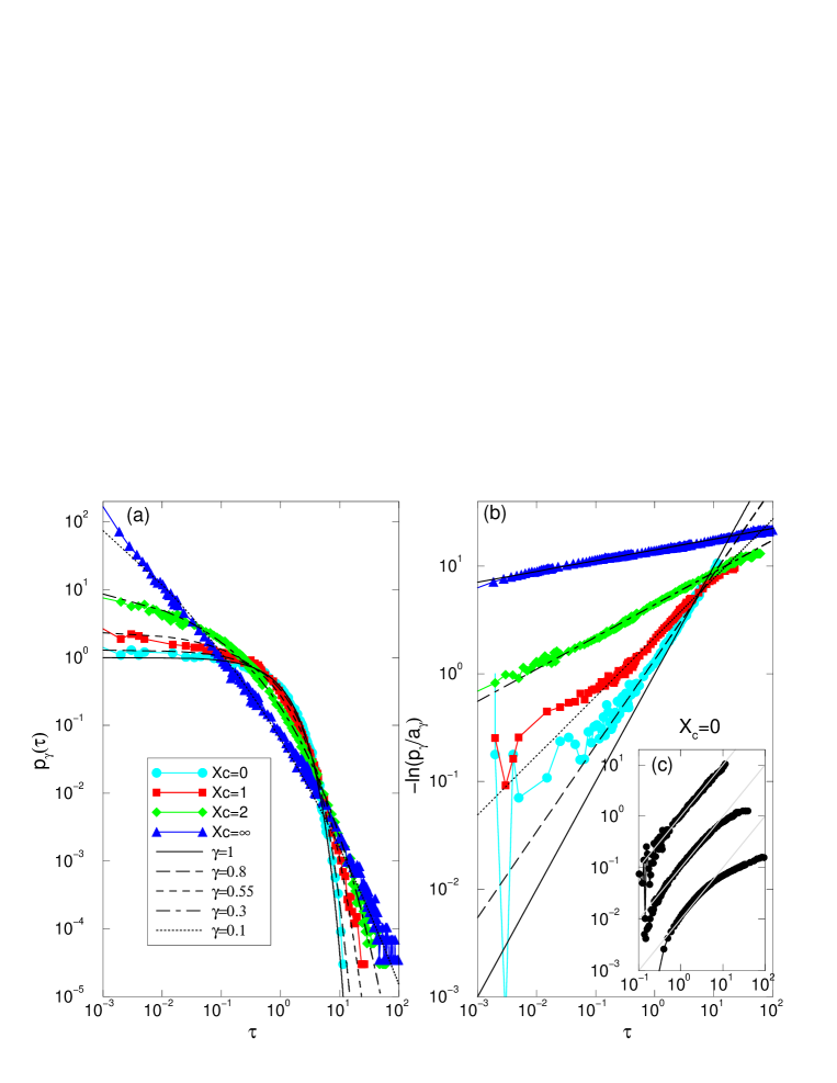
Figure 4: (color online) RTS of long-term correlated linear time series with $\gamma_{c}=0.1$ and different recurrence intervals (centered in $X_{c}$ with measure $\mu(I)=10^{-3}$). The lines are stretched exponentials distributions and the symbols connected by lines are the numerical simulations. From (a) to (b) we use the values given by $a_{\gamma}$ of the best fitting of Eq. (10) in (a). In (c) we analyze the case $X_{c}=0$ for different values of $\mu(I)$, from bottom to top: $\mu(I)=10^{-1}$ (shifted down by $10^{2}$), $\mu(I)=10^{-2}$ (shifted by $10$) and $\mu(I)=10^{-3}$. The gray lines are the Poissonian distribution ($\gamma=1$ in Eq. (10)). $a_{\gamma=1}=1$ was used for all three cases.

Furthermore, we verify in Fig. 4 that, for small $\mu(I)$, the distribution (10) is valid also for recurrence intervals in the inner part of the data range (centered at $X_{c}$ and defined by Eq. (2)). When $X_{c}\rightarrow\infty$, approaching the extreme interval, the value of $\gamma$ in Eq. (10) approaches the value of the correlation exponent $\gamma_{c}$. Decreasing the value of $X_{c}$ towards the mean value of the PDF ($\langle x\rangle=0$) results in an increase of $\gamma$. This case was analyzed carefully in Fig. 4c, where the dependence of the RTS on the size of the recurrence interval $\mu(I)$ is shown. While for big intervals the stretched exponential seems not to hold, when $\mu(I)\rightarrow 0$ (the limit Poincaré was interested in) the distribution for $X_{c}=0$ tends to the upper limit $\gamma=1$, the Poisson distribution.

In summary, the RTS of long-term correlated linear time series with exponent $\gamma_{c}$, in the limit of small interval $\mu(I)\rightarrow 0$, is described by the stretched exponential distribution (Eq. (10)) for all recurrence times $T$ and for recurrence intervals of both types (1) and (2). The exponent $\gamma$ is a continuous and monotonically decreasing function of the center $X_{c}$ of the recurrence interval, with the limits

$$\gamma=\left\{\begin{array}[]{ll}\gamma_{c}&\mbox{when }X_{c}\rightarrow\infty\mbox{ (extreme)},\\ 1&\mbox{when }X_{c}=0.\end{array}\right.$$ (12)

This result has a simple interpretation in terms of the long-term correlations contained in the time series. Calculating the RTS to a specific interval measures the correlation between events inside this interval. In this sense, our result suggests that the long-term correlations of the time series are concentrated in the extreme events (large fluctuations) and vanish for events near the mean value (small fluctuations). Relation (12) can then be interpreted as: approaching pure extreme events ($\mu(I)\rightarrow 0$ and $X_{c}\rightarrow\infty$) the RTS shows the whole correlation and thus $\gamma=\gamma_{c}$. Approaching pure middle events $(\mu(I)\rightarrow 0$ and $X_{c}=0$) no correlation is detected and consequently the Poisson distribution $(\gamma=1)$ is recovered.

III.3 Change of observables

The link between recurrence times on time series and Poincaré recurrences (Sec. I.1) motivates the issue of the change of observables. All of the empirical data exhibiting long-term correlations mentioned before represent systems which involve a huge number of degrees of freedom. Hence, there is a similarly huge arbitrariness in choosing a given observation function $x(\vec{\gamma})$, and the natural question is what to expect when we change this observation function.

For instance, the correlations in the weather can be studied through records of the daily maximum temperature or of the daily precipitation bunde2 . For the first observable, long-term correlations for times larger than $10$ days were found with an exponent $\gamma\approx 0.7$ for continental stations, independent of the location and of the climatic zone of the weather station. On the other hand, the series of precipitation, obtained in the same locations and for the same time windows, are not long-term correlated. A similar situation is observed in financial market data. While the fluctuation of prices are typically uncorrelated the volatility is long-term correlated bouchaud . This gives already a clue that correlations measured on a given time series do in fact characterize the fluctuations of the given observable but do not characterize the underlying system in a more abstract way.

Here we want to study the dependence of correlations and RTS on the chosen observable in more detail by comparing the properties of different observables. Generally, both observables $x$ and $y$ are functions of the $d-$dimensional phase space vectors $\vec{\gamma}$, and no simple function connecting $x$ and $y$ exists. Since we are starting from time series data without underlying multi-dimensional phase space, we will restrict the analysis to a subclass of changes of observables, where in fact $y$ is given by a nonlinear (potentially non-invertible) function of $x$. Hence, we construct time series of different observables $y$ as functions of the original long-term correlated time series of the variable $x$. Having in mind a recurrence interval defined through ($X_{c},\delta$) by relation (2), consider the following reversible transformation

$$y_{n}=\frac{1}{x_{n}-(X_{c}-\delta)},$$ (13)

which is essentially the inverse of the original series $\{x_{n}\}$. If the $x$-series is Gaussian distributed as considered previously, the PDF of the new series $\{y_{n}\}$ is given by

$$\rho^{\prime}(y)=\frac{1}{\sqrt{2\pi}}\frac{1}{y^{2}}e^{-\frac{1}{2}(1/y+(X_{c}-\delta))^{2}},$$ (14)

which is illustrated in Fig. 5 for the case $X_{c}=1,\delta=0.0207$. In this figure it is also shown that the interval $I_{1}$, defined by the same ($X_{c},\delta$) in $x$, is transformed into an extreme interval in $y$. On the other hand, the extreme interval $I_{2}$ in $x$ is transformed into a recurrence interval in the middle of the PDF of $y$. Since the sequence of recurrence times $T$ obtained using the original intervals in the $x$-series is also obtained using the transformed intervals in the $y$-series, the RTS remains invariant under simultaneous transformation of variables and recurrence intervals. Therefore, the previous observation that the change of the recurrence interval in the $x$-series does not affect the functional form of the stretched exponential distribution (10), but does affect the exponent $\gamma$, carries over to transformations of the form (13). For instance, the RTS of a series obtained from transformation (13) applied to a time series $x$ with $\gamma_{c}=0.1$, is well described by the stretched exponential distribution (10) with (see Fig. 4): $\gamma\approx 0.55$ for extreme interval ($I_{1}$ in Fig. 5b) and $\gamma=0.1$ for central interval ($I_{2}$ in Fig. 5). This result holds for all reversible transformations.

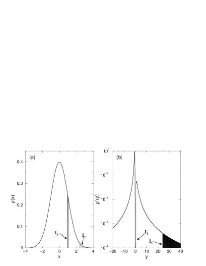
Figure 5: PDF of the series (a) of $x$ (Gaussian) and (b) of $y$ (Eq. (14) with $X_{c}=1,\delta=0.0207$). The points inside the interval $I_{1}(X_{c}=1,\delta=0.0207)$ in $x$ become extreme events in $y$. The opposite happens for the extreme interval $I_{2}=I_{ext}(q=2.3263)$.

An important fundamental question in this context is the behavior of the long-term correlations under transformations of variables. Whereas the normalized autocorrelation function remains unchanged under shifts and rescalings of $x$, this is not the case under transformations like (13), where the transformed time series of $y$ is not long-term correlated at all, despite the long-term correlations of the original $x$-series (see Fig. 6 where $h(2)\approx 0.5$). We characterize the $y$-series using the multi-fractal detrended fluctuation analysis kantelhardt , which is a much more powerful tool than the simple autocorrelation function, since for different values of the parameter $q_{DFA}$ different scales of fluctuations are amplified. In order to distinguish between the multifractality due to long-term correlations and due to a broad PDF, the typical procedure is to shuffle the time series randomly, i.e., we choose randomly a new order of the $N$ points of the original time series. Since the shuffled series loses all its temporal correlations but retains the same PDF, the difference between the results of the two series (original and shuffled) is exclusively due to temporal correlations. In Fig. 6 we show the multi-fractal analysis (MF-DFA1 kantelhardt ) for the long-term correlated, Gaussian distributed, linear time series $\{x_{n}\}$ and for the transformed (through Eq. (13)) time series $\{y_{n}\}$. As expected, in the first case roughly a single generalized Hurst exponent $h(s)$ is obtained for all scales in the original ($h(s)=1-\gamma_{c}/2=0.95$) and shuffled ($h(s)=0.5$) time series. Due to the broad tails present in Eq. (14), both the $y$-series and its shuffled version have multi-fractal spectrum, shown by the nontrivial dependence of $h(q_{DFA})$ on $q_{DFA}$. The difference between the two, which measures the effect of the temporal correlations, appears for small scales, where the generalized Hurst exponent of the shuffled series is smaller. This result is consistent with the interpretation made at the end of Sec. III.2 that the correlations of the $x$-series is concentrated on the extreme events. Through transformation (13), the extreme events in $x$ are mapped into very small fluctuations in $y$ and the temporal correlations of $\{y_{n}\}$ are coherently noticeable for small values of $q_{DFA}$.

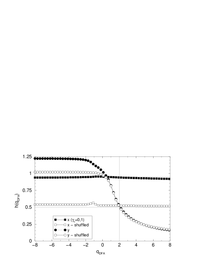
Figure 6: Generalized Hurst exponent of the time series of $x$ and $y$ ($N=2^{20}\approx 10^{6}$ points) as a function of the scale $q_{DFA}$. The horizontal gray lines are the non-correlated value ($h=0.5$) and the expected value for $\gamma_{c}=0.1$ ($h=1-\gamma_{c}/2=0.95$). The difference between the original and the shuffled time series measures the effect of the correlation at each scale $q_{DFA}$.

Through transformation (13) we provide an example of equivalence between the RTS of different observables obtained using extreme intervals, and the RTS calculated in the same series but using different recurrence intervals. Always when the transformation of observables is invertible, there exist a one-to-one correspondence between the original extreme values and a new interval. This provides another justification to the generalization of the recurrence of extreme events to general recurrence intervals, proposed in Sec. I.1 inspired by the analogy to the Poincaré recurrences.

III.4 The series of recurrence times

It is also interesting to apply the distinction between the time properties of the series and its PDF, discussed in Sec. II, to the series of recurrence times $\{T_{1},T_{2},...T_{Ne}\}$ itself multifractal . In this case this means that the PDF, which is the RTS of the original time series, is independent of its correlation and shows that the results (ii) and (iii) stated in Sec. I.3 are independent. This is an important remark when prediction algorithms are considered, since in many cases the correlation between the waiting times is more important than their distribution mega.prl .

The result (iii) of Ref. bunde is verified in Fig. 7 through the multifractal analysis of the series of recurrence times $T$. Instead of the same correlation exponent we find a multifractal spectrum. It is necessarily originated by the long-term correlations since the PDF of these series are stretched exponential distributions, as verified in Fig. 4, which do not have fat tails.

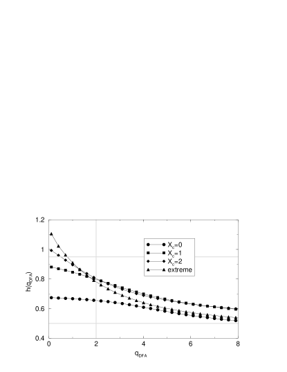
Figure 7: Multifractal spectrum for the series of recurrence times $(\{T_{1},T_{1},...,T_{Ne}\})$ obtained for intervals with $\mu(I)=0.01$, and different values of $X_{c}$ in long-term correlated linear time series with $\gamma_{c}=0.1$ ($N_{e}=2^{18}\approx 2\;\times 10^{5}$).

IV Discussion and Conclusion

Well established regimes of decay of the RTS are exponentials and power-laws, and, only recently observed, stretched exponentials. We have obtained a closed expression for the stretched exponential distribution of recurrence times uniquely defined by the exponent $\gamma$. As limits $\gamma=1$ and $\gamma=0$, respectively, we recover the exponential and the power-law decay from these (with the restriction that the power is fixed to 3/2), suggesting that stretched exponentials describe recurrences in systems that have neither exponential nor power-law RTS but that lie in between these two cases. We have verified numerically that the stretched exponential distribution is in good agreement with the numerical results obtained for long-term correlated linear time series, similarly to what was done in Ref. bunde . From the point of view of these previous results, listed in Sec. I.3, we have identified (i) with Kac’s lemma; generalized (ii) to the stretched exponential distribution (10), which is a function of a single parameter and is valid for all recurrence intervals through Eq. (12); and generalized (iii), showing that the sequence of recurrence times has a multi-fractal spectrum, with an exponent $\gamma_{T}$ different from $\gamma_{c}$. In order to verify if the fluctuations around the stretched exponential distribution, shown in the figures of Sec. III.2, are a consequence of numerical limitations or real deviations, an analytical deduction of the stretched exponential distribution (10) is necessary, what remains an open task.

Performing simple reversible transformations (like Eq. (13)) on the original long-term correlated linear time series $\{x_{n}\}$, we have shown that the stretched exponential distribution characterizes also the RTS of extreme events in time series that are not long-term correlated. The presence and absence of long-term correlations in the series of the original observable $x$ and of the transformed observable $y$, respectively, is similar to the one reported above for climatic records (temperature and precipitation) and stock-market indexes (volatility and fluctuation of price). It is remarkable that this interesting behavior is obtained already through the simplest possible approach, i.e., two different observables that depend directly and exclusively on each other. These considerations emphasize that the temporal characterization of the system through the autocorrelation or RTS depend crucially on the chosen observable. By analyzing both the dependence of the exponent $\gamma$ of the stretched exponential distribution with the center of the recurrence interval (relation (12)) and the multi-fractal spectrum of the $y$-series (FIG. 6) we conclude that, in long-term correlated linear time series, the correlations are concentrated in the extreme events.

Many interesting questions arise if one supposes that the measurements in a given experiment lead to the time series of the observable $y$, introduced in Sec. III.3, and that no natural access to the observable $x$ exists. The $y$-series has a complex multi-fractal spectrum (Fig. 6), a strange PDF (Eq. (14)) and a non-trivial dependence of the RTS with the recurrence interval. Nevertheless, through a simple transformation (the inverse of relation (13)) one arrives at the $x$-series, that has a mono-fractal spectrum, is Gaussian distributed and has a simple (Eq. (12)) dependence of the RTS on the recurrence interval. This suggests the existence, in some situations, of “distinguished observables” where the time series analysis is extremely simplified. It is an interesting open problem to develop a procedure able to determine the transformation (when it exists) that lead to the “distinguished observables”.

- (1) A. Bunde, J. F. Eichner, S. Havlin, and J. W. Kantelhardt. Physica A, 330:1, 2003.
- (2) A. Bunde, J. F. Eichner, J. W. Kantelhardt and S. Havlin. Phys. Rev. Lett., 94, 048701 (2005).
- (3) A. Bunde, J. Eichner, R. Govindan, S. Havlin, E. Koscielny-Bunde, D. Rybski, and D. Vjushin. In Nonextensive Entropy-Interdisciplinary Applications. (Oxford Univ. Press, New York, 2003). arXiv:physics/0208019.
- (4) M. S. Santhanam and H. Kantz. Physica A, 345: 713, 2005.
- (5) To associate the recurrence time with residence time in stochastic resonances see R. B. Alley, S. Anandakrishnan, and P. Jung. Paleoceanography, 16(2):190, 2001.
- (6) P. Bak et al. Phys. Rev. Lett., 88(17):178501, 2002; A. Corral. Phys. Rev. Lett., 92(10):108501, 2004; N. Scafetta and B. J. West. Phys. Rev. Lett., 92(13):138501, 2004; J. Davidsen and C. Goltz Geophys. Res. Lett., 31:L21612, 2004.
- (7) G. Boffetta et al. Phys. Rev. Lett., 83(22):4662, 1999.
- (8) J. Davidsen and H. G. Schuster. Phys. Rev. E, 65:026120, 2002.
- (9) M. S. Baptista, I. Caldas, M. Heller, and A. A. Ferreira. Physics of Plasmas, 8:4455, 2001.
- (10) M. S. Baptista and I. L. Caldas. Physica A, 312:539, 2002.
- (11) E. G. Altmann, E. C. da Silva, and I. L. Caldas. Chaos, 14(4):975, 2004.
- (12) M. Kac. Bulletin of the American Mathematical Society, 53:1002, 1947.
- (13) G. M. Zaslavsky. Physics Reports, 371:461, 2002.
- (14) A. Sornette and D. Sornette. Europhys. Lett., 9(3):197, 1989.
- (15) X. Yang, S. Du, and J. Ma. Phys. Rev. Lett., 92(22):228501, 2004.
- (16) K. Christiansen and Z. Olami. J. Geophys. Res., 97(B6):8729, 1992.
- (17) R. Sánchez, D. E. Newman, and B. A. Carreras. Phys. Rev. Lett., 88(6):068302, 2002.
- (18) M. Hirata. Ergod. Th. Dyn. Systems, 13(3):533,1993. Hirata et al. Comm. Math. Phys., 206:33,1999.
- (19) J. W. Kantelhardt, S. A. Zschiegner, E. Koscielny-Bunde, S. Havlin, A. Bunde, and H. E. Stansley. Physica A, 316:87, 2002.
- (20) S. Thurner et al. Fractals, 5(4):565, 1997. arXiv:adap-org/9709006.
- (21) S. Prakash, S. Havlin, M. Schwartz, and H. E. Stanley. Phys. Rev. A, 46(4):R1724, (1992).
- (22) G. E. P. Box, G. M. Jenkins, and G. C. Reinsel. Time series analysis : forecasting and control (Prentice Hall, New Jersey, 1994).
- (23) J. Davidsen and M. Paczuski. Phys. Rev. E, 66:050101(R), 2002.
- (24) M. Potters, R. Cont, and J. Bouchaud. Europhys. Lett., 41(3):239, 1998.
- (25) The (multi-) fractal properties of the recurrence times were studied from different perspectives in: V. Afraimovich and G. M. Zaslavsky, Phys. Rev. E, 55 (5):5418 (1997) and N. Hadyn et al. Phys. Rev. Lett., 88 (22):224502 (2002).
- (26) M. S. Mega et al. Phys. Rev. Lett., 90(18):188501, 2003.