High order stimulated Brillouin scattering in single-mode fibers with strong feedback

Abstract

We present an experimental and theoretical study of cascaded high order Stimulated Brillouin Scatterings (SBS) in single mode fibers. It is shown that because of the back-scattering nature of the process, feedback in the input port is needed for obtaining a significant cascaded effect in nonresonant systems. We also discuss similarities to nonlinear photorefractive processes.

I Introduction

Stimulated Brillouin Scattering (SBS) has a long research history as a basic phenomenon and as a tool in many contexts and materials. We mention here two important connections to SBS that were intensively studied in the last three decades. The first one is the link to phase conjugation zeldovich . It was found that the reflection of focused light beams in various media gave in some cases a phase conjugate replica of the input beam. This method gave maybe the first demonstration of phase conjugation, and later generated many activities. Another wave of research was related to SBS in fibers agrawalbook , first in multi-mode fibers, and then more intensively to single mode fibers. Here the conventional meaning of phase conjugation in the spatial or pictorial aspect is meaningless, especially when we consider single mode fibers. Nevertheless, the nonlinear coupling efficiency becomes very high even for low light powers at the mW regime, due to the light confinement along large distances in the fiber, compared to limited focused lengths that can be obtained in free space propagation. Therefore, SBS became a crucial factor that has to be considered in fiber-optic communications. It is usually an effect that must be eliminated to allow the light propagation without losing a big fraction of it to reflections. It is similar to another effect that was used for phase conjugation, the stimulated Raman scattering (SRS). In the SRS case however, there were found important uses in fiber-optic communications. The main one is the use as broadband amplifiers, especially at the important $1.5\mu m$ wavelength regime. A difference between SRS and SBS is the magnitude of the frequency shift of the reflected light (Stokes wave) compared to the input, originating from the vibration frequency of the relevant medium entity involved in the nonlinear process. This frequency shift is in fibers on the order of $~{}10GHz$ for SBS and $~{}13THz$ in fibers for SRS at the $1.5\mu m$ wavelength regime.

In this paper we focus our attention on a cascaded SBS process in single-mode fibers. Therefore the present work doesn’t offer any direct use for phase conjugation. Nevertheless, it can be meaningful for other SBS schemes, in free space and multi-mode fibers, where ”spatial” phase conjugation is applicable. Additionally, one might find possible applications by using the self frequency shifts that are in the order of future dense WDM (wavelenght division multiplexing) technologies, believed to be heavily used in future fiber-optic communications.

For this paper, presented in the context of works on dynamic holography and photorefractive optics, it is worthwhile to mention some similarities between SBS, SRS and photorefractive four-wave mixing. Pioneering work was done at the early stages when photorefractive materials have been started to be a part of the field of nonlinear-optics, and was used for wave mixing, phase conjugation and oscillators, at a few places around the world: in Kiev Kiev (by Kukhtarev, Markov, Odulov, Soskin, and Vinetskii), at Thomson CSF Huignard (by Huignard, Spitz, Aubourg, and Herriau, at the University of Southern California Feinberg (by Feinberg and Hellwarth), and at Caltech PR0 ; PR1 (by Cronin-Golomb, Fischer, White and Yariv. Later, a huge stream of research was done around the world in many aspects of photorefractivity. We mention a few works on photorefractive wave-mixing, done in our group at Technion PR2 ; PR3 ; PR4 ; PR5 ; PR6 ; PR7 ; PR8 ; PR9 (by Fischer, Sternklar, Weiss and Segev), that can be associated to the present work on SBS. The first link is to a class of self oscillation processes in photorefractive media Feinberg ; PR1 ; PR2 . Like in SBS, passive or self-pumped phase conjugate mirrors can be obtained. Here four-wave mixing PR3 ; PR4 gives spontaneous phase conjugate reflection via pump beams which are self generated and can be regarded as the ”internal” crystal ”waves” (albeit light waves), like the self generated ”sound waves” in the SBS case zeldovich . The phase conjugation property can be also explained by similar arguments, that among all possible scattering, the phase conjugate pattern which is an oppositely propagating replica of the input light wave (and therefore coincide in space), experiences the highest gain, and thus wins out and prevails over all other scatterings zeldovich ; PR5 ; PR6 . Another similarity is the self frequency shift of the reflection with respect to the input light beam PR7 ; PR8 ; PR9 . In the photorefractive case, the shift is typically in the $1-10^{-3}Hz$ region, depending on the photorefractive buildup time constant, which is much slower that the relevant nonlinear effect in the SBS and SRS cases. Additionally, for photorefractive wave mixing one can also think of cascaded self reflections in an open or closed cavity. Specific examples can be two-beam coupling, via reflection gratings where the beams are almost counter-propagating, or resonators that give high order oscillations.

It is also worthwhile to mention connections of fibers to phase conjugation. In fact, one of the first suggestions for methods of phase conjugation and its uses dealt with the restoration of images transmitted through multi-mode fibers PC1 . It was proposed there to use nonlinear three-wave mixing to phase conjugate the distorted image transmitted through a fiber, and retransmit it through an identical fiber section, such that the second propagation exactly cancels the phase distortion of the first section. The idea was later demonstrated PC2 in a single section fiber with a round-trip propagation in the same fiber, because of the difficulty to get two identical multi mode fibers. Another idea in the early stages of research that gained a lot of recent attention in the fiber-optic communication community was to compensate for dispersion in single mode fibers by using the phase conjugation property of flipping the spectral band of a time dependent signal PC3 . Again a two section scheme with phase conjugation between them, can provide a perfect compensation.

SBS in fibers has been studied intensively throughout the years. Input light at power levels on the order of 10 mW is strongly backscattered, producing a frequency down shifted Stokes wave, due to nonlinear interaction of light and sound waves. The associated threshold depends on the light losses. The simplest configuration for studying SBS in optical fibers is just a long enough optical fiber, typically of a few km, with a good termination at its far end, to avoid feedback. Much work has been done analyzing this system, the SBS threshold feedback and the reflection strength, which is the ratio between the final power of the Stokes wave and the initial power of the pump.

When feedback is added to the fiber from the far end termination, or from other reflectors or simply by forming a ring cavity, the SBS threshold can be lowered significantly and can even result in oscillation and a Brillouin laser.

In a fiber with no feedback, SBS is well described by the common ”three wave model”: the pump wave, the Stokes wave and the mediating sound wave. Second order SBS 2order , which is the generation of yet another, secondary Stokes wave, by SBS from the first SBS wave, is known but considered to be weak for systems without gain, and is usually neglected for such systems. However, for systems with strong feedback, higher SBS orders can be significant, and taking them into account is crucial for understanding the physics of such systems.

In this work we investigate a system with strong feedback, where several orders, a cascade of SBS, are generated, in a non-resonant system (open cavity, with only one side feedback ). We realize that it is necessary to put the feedback at the input port of the fiber to allow the each SBS backscattering order to generate its own SBS in an optimized intensity profile along the fiber interaction path. We compare the experimental results to theoretical analysis, and trace clearly the vast effects of second and third order SBS. We find good agreement between the experimental data and the multiple-order SBS theory.

II SBS without feedback

In the simple Brillouin scattering scheme in long fibers most of the energy of the input laser can be transferred to the Stokes wave. Therefore one would expect that the Stokes wave would pass its energy to a counter propagating Stokes wave moving again in the direction of the input laser beam, and with a frequency of $\omega_{0}-2\Omega$. Then one can ask if and what order can be reached in such a chain of cascaded SBS system? (the n-th order having an additional frequency shift, such that $\omega_{0}-n\Omega$.) We will mathematically solve the coupled wave equations for these three waves and then show experimentally that for a regular system, even the generation of the second order (third wave) SBS is negligible. Later we show that a chain process that builds many strong high order SBS is possible by adding feedback via a simple reflector at the input port.

The common three-wave SBS model (one acoustic and two light waves) in steady state, is described by two coupled differential equations, for the intensities of the pump and the Stokes wave boydbook :

$$\frac{dI_{1}}{dz}=-gI_{1}I_{2}$$

$$\frac{dI_{2}}{dz}=-gI_{1}I_{2},$$ (1)

where $I_{1}$ and $I_{2}$ are the intensities of the incident and the Stokes waves respectively. $g$ is the Brillouin gain parameter, that depends on the fiber. These equations neglect losses in the fibers and can be integrated analytically (as well as the ones with nonzero losses Chen ) to yield the following intensity profiles:

$$I_{2}(z)=\frac{I_{2}(0)(I_{1}(0)-I_{2}(0))}{I_{1}(0)e^{gz(I_{1}(0)-I_{2}(0))}-I_{2}(0)}$$ (2)

(3)

$$I_{1}(z)=I_{1}(0)-I_{2}(0)+I_{2}(z)$$ (4)

We choose our origin $z=0$ at the pump input port of the fiber. Then $I_{1}(0)$ is the intensity of the incident wave, and $I_{2}(0)$ is the output intensity of the Stokes wave.

It is seen that if $I_{2}(L)$, the intensity of the Stokes wave at the far side of the fiber, is zero, then $I_{2}(z)\equiv 0$, which means that there is no Stokes wave at all. This reflects the fact that the Stokes wave must start from a seed, whose source is noise in the system. According to several approaches boyd1 ; boyd2 , it is important to think of the noise as distributed all over the fiber. We shall follow here the simple case of a noise seed at the far side of the fiber, on the order of 1nW.

Requiring $I_{2}(L)=\varepsilon$ in (2) yields a relation between the incident power $I_{1}(0)$ and the power of the Stokes wave $I_{2}(0)$ in terms of a transcendental equation. We shall denote this relation by

$$I_{2}(0)=B(I_{1}(0)).$$ (5)

The function $B$ can be approximated, for low input intensities, by

$$I_{2}(0)=\varepsilon e^{gLI_{1}(0)}$$ (6)

This approximation is good as long as $\varepsilon e^{gLI_{1}(0)}<<I_{1}(0)$ i. e. for small enough incident intensities $I_{1}(0)$, and can be obtained as well by the non-depleted pump approximation.

Equations (1) neglect losses in the fiber. One of the outcomes of losses in the fiber is the existence of a threshold for SBS. It starts only if the incident beam is intense enough. Otherwise, losses suppress the Stokes wave. Moreover, the transfer of energy from the incident beam to the Stokes wave lasts only while the intensity of the incident wave remains above the threshold. Losses are also known to shorten the effective length of the fiber, so the physical length in 6 is replaced by an effective length agrawalbook

$$L_{eff}=\frac{1}{\alpha}(1-e^{-\alpha L}),$$ (7)

where $\alpha$ is the fiber loss coefficient.

Second order SBS requires a three optical wave model. The coupled wave equations for the intensities are given by 2order ; boydbook :

$$\frac{dI_{1}}{dz} = -gI_{1}I_{2}$$ (8)

$$\frac{dI_{2}}{dz} = -gI_{1}I_{2}+gI_{2}I_{3}$$ (10)

$$\frac{dI_{3}}{dz} = gI_{2}I_{3}$$ (12)

$I_{1}$ the incident wave, $I_{2}$ the back scattered Stokes wave, $I_{3}$ the Stokes wave generated by $I_{2}$, which propagates in the same direction as $I_{1}$, etc. For three optical waves the equations can be integrated analytically 2order , but unfortunately the three integration constants appearing in the solution are again transcendental functions of the boundary conditions. One can easily verify that

$$C_{1}=I_{1}-I_{2}+I_{3}\quad{\rm and}\quad C_{2}=I_{1}I_{3}$$ (13)

are constants of motion. Then we can find that

$$I_{1}(z)=\frac{C_{1}}{2}+(\frac{q}{2})\frac{1+C_{3}e^{-qz}}{1-C_{3}e^{-qz}};\quad q=\sqrt{C_{1}^{2}-4C_{2}}$$ (14)

$C_{3}$ is the third integral, and $I_{2}(z),I_{3}(z)$ can be obtained from 14 through 13

In spite of the similarity of the terms $gI_{1}I_{2}$ and $gI_{2}I_{3}$ in 8, power exchange between $I_{1}$ and $I_{2}$ is much more efficient than between $I_{2}$ and $I_{3}$. The difference stems form the boundary conditions. For a system without feedback $I_{3}$ has the initial value of $\varepsilon$ at $z=0$ and grows as $z$ increases, whereas $I_{2}$ decays as $z$ increases, keeping their product small all the way to $z=L$.

For a system without feedback or gain, the second order SBS is weak compared to the pump and to the first order SBS. Indeed, from the second relation of Eq. 13 one obtains

$$I_{3}(z)=I_{1}(0)\frac{\varepsilon}{I_{1}(z)}$$ (15)

Since $I_{1}(0)$ and $I_{1}(z)$ are roughly of the same order of magnitude, one concludes that the second order SBS $I_{3}(z)$ is not high above the noise level $\varepsilon$.

To verify Eq.(15), we measured $I_{3}$ using a very simple experimental setup shown in Fig. 1. The fiber we used was SMF-28, of 25 kilometers long. The output spectrum at $Z=L$, shown in Fig. 2, is composed of three wavelengths, $I_{3}(L),I_{1}(L)$ and the reflections from the input isolator of the first Stokes wave $I_{2}$. In Fig. 3 we have plotted $I_{3}(L)$ vs. $I_{1}(0)$ . In the range of input intensities we have applied, $I_{1}(L)$ was weakly dependent on $I_{1}(0)$ and was about 1.5mW. We observe that $I_{3}(L)$ changes linearly with $I_{1}(0)$ as expected from Eq. (15). The slope can be related to $\varepsilon$ to yield $\varepsilon\approx 1nW$.

Figure 1: Experimental setup (regular - without feedback elements) for examining SBS .

Figure 2: Optical spectrum of a simple SBS process.

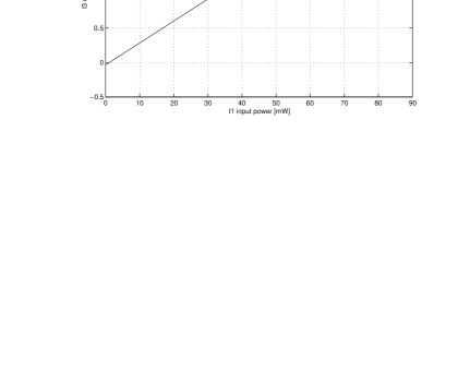
Figure 3: Output power of second stokes $(I_{3})$ vs. the input power $(I_{1})$ for a double SBS process without feedback.

We thus summarize that a cascaded SBS beyond the first order SBS without feedback elements is very weak. Nevertheless we show below that with proper boundary conditions with one reflector, strong higher order SBS can be generated.

III System with feedback and high order SBS

We have seen that the Stokes waves generated by SBS don’t generate their own Stokes waves because of the opposite growth direction along the fiber of the ”pump” and its SBS product. One way to cascade many Brillouin scattered waves is by intervening in the setup, causing every set of waves to resemble a two wave system. Fig. 4 represents a suggested setup we check experimentally. The input laser beam enters the system through a fiber Bragg grating. The initial wave that start the cascading process is obtained at the output of the grating. We will denote this wave as $I_{1}$. It propagates to the right, generates a Stokes wave $I_{2}$ that propagates to the left. We know that $I_{2}$ doesn’t generates its own Stokes, however when $I_{2}$ is reflected back from the grating it will create a Stokes wave travelling again to the left, since after the reflection the waves $I_{3}$ and $I_{4}$ behave according to the two wave system equations. $I_{3}$ begins with a large power at the Bragg grating and is depleted only by its Stokes wave $I_{4}$, which means that the coupled equations for two waves can be used. This behavior is repeated for $I_{3}$ and $I_{4}$, $I_{5}$ and $I_{6}$ and so on. From understanding how this system works we can easily conclude that the coupling between every pair of waves is only through the boundary conditions of each pair. For the first pair the known boundary conditions are given by $I_{1}(0)$ and $I_{2}(l_{eff})$, and for the second pair by $I_{2}(0)$, which is the solution of the first pair, and by $I_{3}(l_{eff})$ and so on. Each pair of waves gets it boundary condition from the solution of the previous pair.

We first present the experimental result showing the generation of strong high orders. The experimental setup is given in Fig. 5. We used a 25km long single-mode fiber. Since every Stokes wave is down shifted by 10.3GHz from its ”pump”, we used a broadband Bragg grating which can reflect all the Stokes waves with approximately the same reflectivity. Knowing the input power to our system and the reflection function of the grating is sufficient to calculate the output spectra of both output1 and output2. We expect to obtain at output port 2 a multiple-peaks spectrum, with a 10.3GHz spacing, each of power $I_{th}$, since we took a long enough fiber for the incident wave to be exhausted down to the SBS threshold power. At output port 1 we should also see a multiple-peaks spectrum. The first peak is due to the direct reflection from the Bragg grating of the input laser with power of $I_{in}\cdot r$, and all the rest are the back scattered Stokes waves. In Figs. 6,7 we show the output spectra from ports 1 and 2. The central four strong lines belong to the input and the first three SBS orders. We can see additional two weaker lines at the right side giving the 4th and 5th SBS orders, and at outpot port 2 additional three four-wave mixing products, resulting mainly from the mixing of the input wave with the strong first SBS orders.

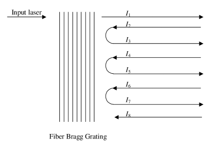
Figure 4: Cascaded SBS setup.

For the theoretical part we write the coupled wave equations. We solved numerically the equations for the first eight waves in the system and compared them to the experiment.

The coupled equations for the eight waves are:

$$\frac{dI_{1}}{dz} = -gI_{1}I_{2}$$ (16)

$$\frac{dI_{2}}{dz} = -gI_{1}I_{2}+gI_{2}I_{5}$$ (18)

$$\frac{dI_{3}}{dz} = -gI_{3}I_{4}$$ (20)

$$\frac{dI_{4}}{dz} = -gI_{3}I_{4}+gI_{4}I_{7}$$ (22)

$$\frac{dI_{5}}{dz} = -gI_{5}I_{6}+gI_{2}I_{5}$$ (24)

$$\frac{dI_{6}}{dz} = -gI_{5}I_{6}$$ (26)

$$\frac{dI_{7}}{dz} = -gI_{7}I_{8}+gI_{4}I_{7}$$ (28)

$$\frac{dI_{8}}{dz} = -gI_{7}I_{8}$$ (30)

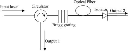
Figure 5: Experimental arrangement for multi stage SBS.

Figure 6: Output spectra of multi stage SBS measured at output 1.

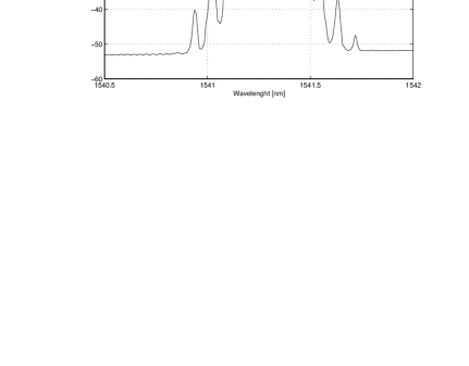
Figure 7: The experimental output spectrum of multi order SBS measured at the output port 2.

We note that the all SBS orders (even $n$ waves) are generated as they propagate to the left direction, but then they are reflected by the mirror at the left (input) side. This reflection enables the cascaded process by generating the SBS. Thus the definition of the eight wave used in the equations is as follows:
$I_{1}$: frequency $\omega$ propagating to the right.
$I_{2}$: frequency $\omega-\Delta\omega$ propagating to the left.
$I_{3}$: frequency $\omega-\Delta\omega$ propagating to the right.
$I_{4}$: frequency $\omega-2\Delta\omega$ propagating to the left.
$I_{5}$: frequency $\omega-2\Delta\omega$ propagating to the right.
$I_{6}$: frequency $\omega-3\Delta\omega$ propagating to the left.
$I_{7}$: frequency $\omega-3\Delta\omega$ propagating to the right.
$I_{8}$: frequency $\omega-4\Delta\omega$ propagating to the left.

For the boundary conditions we have at the left side ($z=0$) the reflectivity ratio $r$ between waves $I_{3}\,\&\,I_{2}$, $I_{5}\,\&\,I_{4}$ and $I_{7}\,\&\,I_{6}$, and at the right side ($z=L$) the thermal noise ($I_{2},I_{4},I_{6}\&I_{8}$) needed for the SBS. Thus:

$$I_{1}(z=0)=I_{p}$$ (31)

$$I_{n}(z=L)=\varepsilon\phantom{I_{n}}\quad\,for\,n=2,4...$$ (32)

$$I_{n}(z=0)=rI_{n-1}\quad\,for\,n=3,5...$$ (33)

We don’t elaborate here on the simulation results, that will be given elsewhere, but note that they show a plausible match, although not complete, to the experiments. There remains questions and ingredients that have to be considered. An important point is the way that the seeding noise is incorporated into the system. In a realistic model it should be taken as a stochastic source distributed along the fiber. Additionally, other elements, such as four-wave mixing and losses, should be included in some cases in the calculations.

IV Brillouin Laser

Understanding the simple cascading process for the multiple Stokes waves can lead to a much more efficient setup for creating the multi wavelength comb of Brillouin Stokes waves. The setup, shown in Fig. 8 is in the form of a long laser with feedback in both sides of the cavity, and an external injected seed to start the scattering process.

Figure 8: Experimental setup for a Brillouin laser.

When the laser operates without the externally injected signal its spectrum is governed only by the reflectivity spectrum of both gratings, but when we start injecting an external laser source through one of the gratings a process similar to the process in the multi Stokes system happens and multi SBS Stokes appear. In the laser configuration the Stokes waves have feedbacks on both sides and the Stokes are travelling in an amplifying media, therefore they are amplified inside the cavity which gives the potential ability for many more Stokes waves. The In this configuration, of course, light is generated only in longitudinal modes which meet the cavities longitudinal mode restriction, but in a long cavity with relatively narrow spaced modes we see all the Brillouin Stokes waves develop. In addition to the high order SBS it is also possible to have products of four-wave mixing (4WM). Every two SBS waves, can generate a new wave by 4WM. The result are waves with the same frequency spacing, but here also with a possible positive frequency shift; thus also getting new lines with higher frequencies (or lower wavelengths).

In Fig. 9 we show the output of the Brillouin laser described above. Comparing the spectrum of the Brillouin laser to that of the multi Stokes open system (Fig. (7) we see the numerous number of Brillouin lines and also the lines generated by four-wave mixing (4WM), especially those above the input frequency.

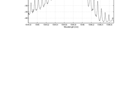
Figure 9: The experimental Brillouin laser output spectrum.

In this experiment we used a chirped grating for one of the ’mirrors’ and deliberately chose a grating that compensates for the dispersion of one round trip in the laser, this selection increased the amplitude of the 4WM terms compared to the same laser with a non-chirped grating, but had no effect on the terms created by SBS. We tested this view to show that SBS terms are phased matched and that the peaks we see are mostly SBS and not other non-linear phenomena.

V Discussion and Summary

We have demonstrated that the SBS process does not cascade by itself in open system configurations due to the power profile of the waves in optical fibers. In order to cascade the SBS process we must intervene in the system to change the basic configuration of the interacting waves. One way of achieving this is by the use of a Bragg reflector which changes the power profile to be favorable for the generation of higher stokes reflection. In this simple setup each pair of waves, signal and its Stokes, can be treated as a simple SBS reflection and all pairs are related through the boundary conditions of the setup. The boundary condition relations make it simple to design the output power of each Stokes wave by changing the input power and the Bragg reflector’s reflectivity. We have also demonstrated a closed system of a laser configuration which is much more efficient than the non-feedback setup and can generate many more SBS reflections, but is not as simple to analyze and design.

References

- (1) B.Ya. Zel’Dovich, N.F. Pilipetsky, V.V. Shkunov, Principles of Phase Conjugation, Springer Series in Optical Sciences, 42 , 1985.
- (2) G. P. Agrawal, Nonlinear Fiber Optics, Academic Press, Second Edition, 1995.
- (3) N. V. Kukhtarev, V. B. Markov, S. G. Odulov, M. S. Soskin, V, L. Vinetskii, ” Holograpghic Storage in Electrooptic Crystals 1@2. Steady State and Beam Coupling - Light Amplification; Ferroelectrics 22 , 961, 1979
- (4) J. P. Huignard, E. Spitz, P. Aubourg, J.P Herriau, ”Phase-Conjugate Wavefront Generation via Real-Time Holography in rystals”, Opt. Lett. 4 , 21, 1979
- (5) J. Feinberg, R. W. Hellwarth, ”Phase Conjugating Mirror with Continuous-Wave Gain”, Opt. Lett. 5 , 519, 1980
- (6) B. Fischer, M. Cronin-Golomb, J.O. White, and A. Yariv,”amplified reflection, Transmission, and Self-Oscillation in Real-Time Holography”, Opt. Lett. 6 , 519, 1981
- (7) J.O. White, B. Fischer, M. Cronin-Golomb and A. Yariv, ”Coherent Oscillation by Self-Induced Gratings in the Photorefractive Crystal BaTiO3”, Appl. Phys. Lett., 40, 450, 1982.
- (8) B. Fischer, S. Sternklar and S. Weiss, ”Photorefractive Oscillators”, IEEE, J. Quantum Electronics, 25, 550, 1989.
- (9) M. Cronin-Golomb, B. Fischer, J.O. White and A. Yariv, ”Theory and Application of Four Wave Mixing in Photorefractive Materials”, (Invited Paper), IEEE J. Quantum Electr.,QE-20 , 12, 1984.
- (10) S. Weiss, S. Sternklar and B. Fischer, ”Double Phase Conjugate Mirrors: Analysis, Operation and Applications”, Optics Lett., 12, 114, 1987.
- (11) 37. B. Fischer, S. Weiss and S. Sternklar, ”Spatial Light Modulation and Filtering Effects in Photorefractive Wave Mixing”, Appl. Phys. Lett., 50, 483, 1987.
- (12) B. Fischer, S. Sternklar and S. Weiss, ”Photorefractive Laser Oscillation with Intracavity Image and Multimode Fibers”, Appl. Phys. Lett., 48, 1567, 1986.
- (13) B. Fischer, ”Theory of Self Frequency Detuning of Oscillators by Wave Mixing in Photorefractive Crystals”, Optics Lett., 11, 236, 1986.
- (14) S. Sternklar, S. Weiss and B. Fischer, ”Tunable Frequency Shift of Photorefractive Oscillators”, Optics Lett., 11, 165, 1986.
- (15) S. Weiss, M. Segev and B. Fischer, ”Line Narrowing and Self Frequency Scanning of Laser Diode Arrays Coupled to a Photorefractive Oscillator”, IEEE, J. Quantum Electronics, JQE, 24, 706, 1988.
- (16) A. Yariv, ”3-Dimensional Pictorial Transmission in Optical Fibers”, Appl. Phys. Lett. 28, 88 1976.
- (17) B. Fischer and S. Sternklar, ”Image Transmission and Interferometry Through Multimode Fibers using Self-Pumped Phase Conjugation”, Appl. Phys. Lett., 46, 113, 1985.
- (18) A. Yariv, D. Fekete and D. Pepper, ”Compensation for channel dispersion by non-linear optical phase conjugation”, Opt. Lett. Vol. 4, 52, 1979.
- (19) M. F. Ferreira, ”Effect of stimulated Brillouin scattering on distributed fibre amplifiers”, Electon. Lett. 30, 40, 1994.
- (20) Alexander L. Gaeta and Robert W. Boyd, ”Stochastic dynamics of stimulated Brillouin scattering in an optical fiber”, Phys. Rev. A 44, 3205, 1991.
- (21) R. W. Boyd and K. Rzazewski, ”Noise initiation of stimulated Brillouin scattering” , Phys. Rev. A 42, 5514, 1990.
- (22) M. Dämmig, G. Zinner, F. Mitschke and H. Welling ”Stimulated Brillouin scattering in fibers with and without external feedback”, Phys. Rev. A 48 , 3301, 1993
- (23) N. Shibata, R. G. Waarts and R. P. Braun, ”Brillouin-gain spectra for single-mode fibers having pure-silica, GeO2-doped, and P2O5-doped cores”, Optics Letters, 12, 269, 1987.
- (24) R. W. Tkach, A. R. Charplyvy and R. M. Derosier, ”Spontaneous Brillouin Scattering for Single-Mode Optical-Fi.bre Characerisation”, Electronics Letters, 22, 1011, 1986.
- (25) R. W. Boyd, Nonlinear Optics, Academic Press, 1992.
- (26) D. Cotter, ”Transient stimulated Brillouin scattering in long single-mode fibres ”, Electronics Letters, 18, 504, 1982; Journal of LightWave Technology, 6, 710, 1988.
- (27) D. S. Lim. H. K. Lee, K. H. Kim, S. B. Kang ,J. T . Ahn and Min-Yong Jeon, ”Generation of multiorder Stokes and anti-stokes lines in a Brillouin erbium-fiber laser with sagnac loop mirror”, Optics Letters, 23, 1671, 1998.
- (28) D. Park, J. Park, N. Park, J. Lee and J. Chang, ”53-line multi-wavelength generation of Brillouin/erbium fiber laser with enhanced Stokes feedback coupling”, OFC (Optical fiber communication) conference, Technical Digest Postconference Edition, 3, 11, 2000
- (29) A. Yariv, Optical Electronics in Modern Communicartions, Oxford University Press, Fifth Edition, 1997.
- (30) L. Chen and X. Bao, ”Analytical numerical solutions for steady state stimulated Brillouin scattering in a single-mode fiber”, Optics Communications, 152, 65, 1998.