Study of the Pioneer anomaly: A problem set

Abstract

Analysis of the radio-metric tracking data from the Pioneer 10 and 11 spacecraft at distances between 20 and 70 astronomical units from the Sun has consistently indicated the presence of an anomalous, small, and constant Doppler frequency drift. The drift is a blueshift, uniformly changing at the rate of $(5.99\pm 0.01)\times 10^{-9}$ Hz/s. The signal also can be interpreted as a constant acceleration of each particular spacecraft of $(8.74\pm 1.33)\times 10^{-8}$ cm/s² directed toward the Sun. This interpretation has become known as the Pioneer anomaly. We provide a problem set based on the detailed investigation of this anomaly, the nature of which remains unexplained.

I Introduction

The Pioneer 10/11 missions, launched on 2 March 1972 (Pioneer 10) and 4 December 1973 (Pioneer 11), were the first to explore the outer solar system. After Jupiter and (for Pioneer 11) Saturn encounters, the two spacecraft followed escape hyperbolic orbits near the plane of the ecliptic to opposite sides of the solar system. (The hyperbolic escape velocities are $\sim$12.25 km/s for Pioneer 10 and $\sim$11.6 km/s for Pioneer 11.) Pioneer 10 eventually became the first man-made object to leave the solar system. See Fig. 1 for a perspective of the orbits of the spacecraft and Tables 1 and 2 for more details on their missions. The orbital parameters for the crafts are given in Table 3.

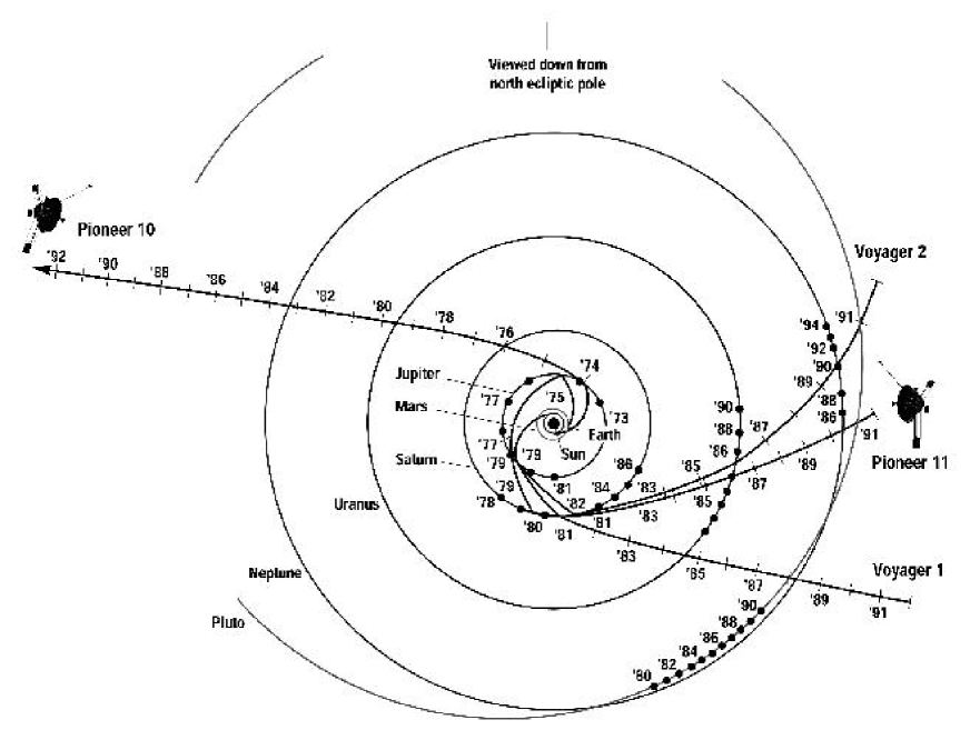
Figure 1: Ecliptic pole view of the Pioneer 10, Pioneer 11, and Voyager trajectories. Pioneer 10 is traveling in a direction almost opposite to the galactic center, while Pioneer 11 is heading approximately in the shortest direction to the heliopause. The direction of the solar system’s motion in the galaxy is approximately towards the top. (Digital artwork by T. Esposito, NASA ARC Image # AC97-0036-3.)

The Pioneers were excellent craft with which to perform precise celestial mechanics experiments due to a combination of many factors, including their attitude control (spin-stabilized, with a minimum number of attitude correction maneuvers using thrusters), power design [the Plutonium-238 powered heat-source radioisotope thermoelectric generators (RTGs) are on extended booms to aid the stability of the craft and also reduce the effects due to heating], and precise Doppler tracking (with the accuracy of post-fit Doppler residuals at the level of mHz). The result was the most precise navigation in deep space to date. See Fig. 2 for a design drawing of the spacecraft.

Table 1: Pioneer 10/11 mission status.

	Pioneer 10	Pioneer 11
Launch	2 March 1972	5 April 1973
Planetary encounters	Jupiter: 4 Dec 1973	Jupiter: 2 Dec 1974
		Saturn: 1 Sep 1979
Last data received	27 April 2002	1 October 1990
at heliocentric distance	$\approx 80.2$ AU	$\approx 30$ AU
Direction of motion	Star Aldebaran	Constell. of Aquila
time to reach destination	$\approx 2$ million years	$\approx 4$ million years

Table 2: Position of Pioneer 10 on 1 January 2005 (data taken from the Jet Propulsion Laboratory’s Horizons system <http://ssd.jpl.nasa.gov/horizons.html>).

Distance from Sun	87.06 AU
Position (lat., long.)	(3.0∘, 78.0∘)
Speed relative to the Sun	12.24 km/s
Distance from Earth	$13.14\times 10^{9}$ km
Round-Trip Light Time	$\approx$ 24 hr 21 min

Table 3: Orbital parameters for Pioneers 10 and 11 at epoch 1 January 1987, 01:00:00 UTC. The semi-major axis is $a$, $e$ is the eccentricity, $I$ is the inclination, $\Omega$ is the longitude of the ascending node, $\omega$ is the argument of the perihelion, $M_{0}$ is the mean anomaly, $f_{0}$ is the true anomaly at epoch, and $r_{0}$ is the heliocentric radius at the epoch. The direction cosines of the spacecraft position for the axes used are $(\alpha,\,\beta,\,\gamma)$. These direction cosines and angles are with respect to the mean equator and equinox of J2000. The ecliptic longitude $\ell_{0}$ and latitude $b_{0}$ are also listed for an obliquity of 23^∘26${}^{{}^{\prime}}$21.${}^{{}^{\prime\prime}}$4119. The numbers in parentheses denote realistic standard errors in the last digits.

Parameter	Pioneer 10	Pioneer 11
$a$ [km]	$-1033394633(4)$	$-1218489295(133)$
$e$	$1.733593601(88)$	$2.147933251(282)$
$I$ [deg]	26.2488696(24)	9.4685573(140)
$\Omega$ [deg]	$-3.3757430(256)$	35.5703012(799)
$\omega$ [deg]	$-38.1163776(231)$	$-221.2840619(773)$
$M_{0}$ [deg]	$259.2519477(12)$	$109.8717438(231)$
$f_{0}$ [deg]	$112.1548376(3)$	81.5877236(50)
$r_{0}$ [km]	$5985144906(22)$	3350363070(598)
$\alpha$	$0.3252905546(4)$	$-0.2491819783(41)$
$\beta$	$0.8446147582(66)$	$-0.9625930916(22)$
$\gamma$	$0.4252199023(133)$	$-0.1064090300(223)$
$\ell_{0}$ [deg]	$70.98784378(2)$	$-105.06917250(31)$
$b_{0}$ [deg]	$3.10485024(85)$	$16.57492890(127)$

By 1980 Pioneer 10 had passed a distance of $\sim$20 astronomical units (AU) from the Sun and the acceleration contribution from solar-radiation pressure on the craft (directed away from the Sun) had decreased to $<4\times 10^{-8}$ cm/s². At that time an anomaly in the Doppler signal became evident and persisted.pioprl Subsequent analysis of the radio-metric tracking data from the Pioneer 10/11 spacecraft at distances between $\sim$20 and 70 AU from the Sun has consistently indicated the presence of an anomalous, small, and constant Doppler frequency drift of $\dot{\nu}=(5.99\pm 0.01)\times 10^{-9}$ Hz/s. The drift can be interpreted as being due to a constant acceleration of the spacecraft of $a_{P}=(8.74\pm 1.33)\times 10^{-8}$ cm/s² directed toward the Sun.pioprd The nature of this anomaly remains unknown, and no satisfactory explanation of the anomalous signal has been found. This signal has become known as the Pioneer anomaly.foot1

Although the most obvious explanation would be that there is a systematic origin to the effect, perhaps generated by the spacecraft themselves from excessive heat or propulsion gas leaks,murphy ; katz ; scheffer none has been found.usmurphy ; uskatz ; mpla Our inability to explain the anomalous acceleration of the Pioneer spacecraft has contributed to a growing discussion about its origin, especially because an independent verification of the anomaly’s existence has been performed.markwardt

Attempts to verify the anomaly using other spacecraft have proven disappointing,pioprd ; mpla ; ijmpd_02 ; Nieto_Turyshev_cqg_2004 because the Voyager, Galileo, Ulysses, and Cassini spacecraft navigation data all have their own individual difficulties for use as an independent test of the anomaly. In addition, many of the deep space missions that are currently being planned either will not provide the needed navigational accuracy and trajectory stability of under $10^{-8}$ cm/s² (that is, recent proposals for the Pluto Express and Interstellar Probe missions), or else they will have significant on-board effects that mask the anomaly (the Jupiter Icy Moons Orbiter mission). The acceleration regime in which the anomaly was observed diminishes the value of using modern disturbance compensation systems for a test. For example, the systems that are currently being developed for the LISA (Laser Interferometric Space Antenna) and LISA Pathfinder missions are designed to operate in the presence of a very low frequency acceleration noise (at the millihertz level), while the Pioneer anomalous acceleration is a strong constant bias in the Doppler frequency data. In addition, currently available accelerometers are a few orders of magnitude less sensitive than is needed for a test. Nieto_Turyshev_cqg_2004 ; ijmpd_02 ; cospar04 ; mexico04 ; stanford04 Should the anomaly be a fictitious force that universally affects frequency standards,pioprd the use of accelerometers will shed no light on what is the true nature of the observed anomaly.

A comprehensive test of the anomaly requires an escape hyperbolic trajectory,pioprd ; mpla ; Nieto_Turyshev_cqg_2004 which makes a number of advanced missions (such as LISA, the Space Test of Equivalence Principle, and LISA Pathfinder) less able to test properties of the detected anomalous acceleration. Although these missions all have excellent scientific goals and technologies, they will be in a less advantageous position to conduct a precise test of the detected anomaly because of their orbits. These analyses of the capabilities of other spacecraft currently in operation or in design lead to the conclusion that none could perform an independent verification of the anomaly and that a dedicated test is needed.Nieto_Turyshev_cqg_2004 ; ijmpd_02 ; cospar04 ; mexico04 Because the Pioneer anomaly has remained unexplained, interest in it has grown.cospar04 ; mexico04 ; stanford04 Many novel ideas have been proposed to explain the anomaly, such as a modification of general relativity, serge ; sanders ; moffat a change in the properties of light,light or a drag from dark matter.foot So far, none has been able to unambiguously explain the anomaly.

The aim of the following problems is to excite and engage students and to show them by example how research really works. As a byproduct we hope to demonstrate that they can take part and understand.

In Sec. II we begin with a few calculations that are designed to provide intuition into the dynamics of the problem. Then we concentrate on the error analysis that demonstrated the existence of the anomaly in the data. In Sec. III we will consider possible sources of errors in the measurement of the Pioneer anomalous acceleration that have origins external to the spacecraft. Section IV will consider likely sources of errors that originate on-board of the spacecraft. We will discuss the anticipated effect of computational errors in Sec. V and summarize the various contributions in Sec. VI. In Appendix A we will discuss the Allan deviation – a quantity useful in evaluating the stability of the reference frequency standards used for spacecraft navigation.

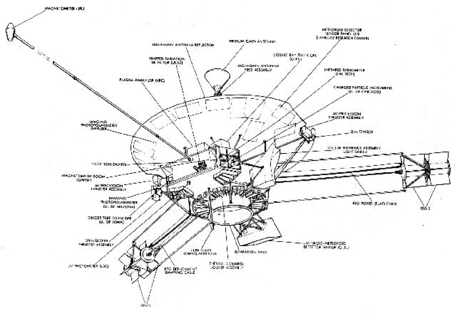
Figure 2: Drawing of the Pioneer spacecraft.

II Effect of the anomaly on the Pioneers’ trajectories

For these problems we can use the approximation of ignoring the angular momentum in the hyperbolic orbits, and treat the velocities as radial.

Problem 2.1. Given the values of the orbital parameters of Pioneer 10 on 1 January 2005 (distance $r_{0}$ and velocity $v_{0}$) in Table 2, what would be the final velocity of Pioneer 10 assuming that there is no anomaly?

Solution 2.1. The terminal escape velocity can be calculated from conservation of energy:

$$v_{\infty}=\sqrt{v_{0}^{2}-2GM_{\odot}/r_{0}}=11.38\,\mathrm{km/s}.$$ (1)

Problem 2.2. Assume that the anomaly continues and is a constant. At what distance from the Sun would the acceleration of the anomaly be equal to that of gravity?

Solution 2.2. We equate the anomalous and Newtonian gravitational forces and find

$$d=\sqrt{GM_{\odot}/a_{P}}\approx 2,600\,\mathrm{AU}.$$ (2)

Problem 2.3. Assume the anomaly is due to a physical force. The time interval over which the Pioneer 10 data was analyzed was 11.5 years (1987 to 1998.5). Because of the anomaly, what is the approximate shortfall in distance which Pioneer 10 traveled during this time?

Solution 2.3. Simple mechanics yields

$$\Delta d=\frac{1}{2}a_{P}t^{2}\approx 57,500\,{\mathrm{km}}.$$ (3)

Problem 2.4. If the anomaly were to continue as a constant out to deep space and be due to a force, how far would Pioneer 10 travel before it reaches zero velocity and starts to fall back in to the Sun? When will the Pioneer reach zero velocity?

Solution 2.4. As seen in Problem 2.1, the gravitational potential energy in deep space due to the Sun is small compared to the kinetic energy of the Pioneer. Therefore, we can ignore it compared to the kinetic energy needed to be turned into potential energy. (This approximation slightly overestimates the time and distance.) If we use the data from Table 2, we can find the time by solving

$$v_{f}=0=v_{0}-a_{P}t.$$ (4)

The solution is $t=1.40\times 10^{13}\,{\rm s}=445,000$ yr. The distance traveled would be given by

$$D=r_{0}+v_{0}t-\frac{1}{2}a_{P}t^{2}\approx 573,300\,\mathrm{AU}=9\,\mbox{light years.}$$ (5)

This distance would be well on the Pioneer 10’s way to Aldebaran (see Table 1). Because this distance is very large compared to $r_{0}=87.06$ AU, this result verifies the validity of the approximation of ignoring the gravitational potential energy.

Problem 2.5. What if the Pioneer anomaly is caused by heat from the RTGs? As stated, they are powered by Plutonium 238, which has a half life of 87.74 years. (See Sec. III for more details on the RTGs.) What would be the change in the final escape velocity of the Pioneers from this cause?

Solution 2.5. The acceleration would be decreasing exponentially due to the radioactive decay of the ²³⁸Pu. Therefore, the change in the velocity would be

$$\Delta v = a_{P}\int^{\infty}_{0}dt~{}\exp[-t(\ln\,2)/(87.74~{}\mathrm{yr})]$$ (6)

$$= a_{P}(87.74~{}\mathrm{yr})/\ln\,2=3.5\,\mathrm{m/s}.$$

III Sources of acceleration noise external to the craft

External forces can contribute to all three vector components of spacecraft acceleration. However, for a rotating spacecraft, such as the Pioneers, the forces generated on board produce an averaged contribution only along the direction of the axis of rotation. The difference in the second case is due to the fact that the two non-radial components (those that are effectively perpendicular to the spacecraft spin) are averaged out by the rotation of the spacecraft. Furthermore, non-radial spacecraft accelerations are difficult to observe by the Doppler technique, which measures the velocity along the Earth-spacecraft line of sight. Although we could in principle set up complicated models to predict effects due to all or each of the sources of navigational error, often the uncertainty of the models is too large to make them useful, despite the significant effort required to use them. A different approach is to accept our ignorance about these non-gravitational accelerations and assess to what extent they could contribute to spacecraft acceleration over the time scales of all or part of the missions.

In this section we will discuss possible sources of acceleration noise originated externally to the spacecraft that might significantly affect the navigation of the Pioneers 10 and 11. We first consider the forces that affect the spacecraft motion, such as those due to solar-radiation pressure and solar wind pressure. We then discuss the effects on the propagation of the radio signal that are from the solar corona, electromagnetic forces, and the phase stability of the reference atomic clocks.

Problem 3.1. There is an exchange of momentum when solar photons impact the spacecraft and are either absorbed or reflected. The models of this process take into account various parts of the spacecraft surface exposed to solar radiation, primarily the high-gain antenna, predict an acceleration directed away from the Sun as a function of the orientation of the spacecraft and its distance to the Sun. The effect of the solar radiation pressure depends on the optical properties of the spacecraft surface (that is, the absorptivities, reflectivities and emissivities of various materials used to build the spacecraft), and the effective areas of the spacecraft part. The effect can be distinguished from the $1/r^{2}$ law due to gravity because the direction between the Sun and the effective spacecraft surface varies.

For navigational purposes, we determine the magnitude of the solar-pressure acceleration at various orientations using Doppler data. The following equation provides a good model for analyzing the effect of solar radiation pressure on the motion of distant spacecraft. It is included by most of the programs used for orbit determination:

$$a_{\rm sp}(r)=\frac{\kappa f_{\odot}}{m\,c}\frac{A\cos\theta(r)}{r^{2}},$$ (7)

where $f_{\odot}=1367\,{\rm W/m}^{2}$(AU)² is the effective Stefan-Boltzmann temperature or solar radiation constant at 1 AU from the Sun, $A$ is the effective area of the craft as seen by the Sun, and $c$ is the speed of light. The angle $\theta$ is the angle between the axis of the antenna and the direction of the Sun, $m$ is the mass of the spacecraft, and $r$ is the distance from the Sun to the spacecraft in AU.

For the Pioneers the effective area of the spacecraft, $A$, can be taken to be the antenna dish of radius 1.37 m. (See Fig. 2 for more information.) The quantity $m$ is the mass of the Pioneers when half of the hydrazine thruster fuel is gone (241 kg). Finally, $\kappa$ in Eq. (7) is the effective absorption/reflection coefficient of the spacecraft surface, which for Pioneer 10 was measured to be $\kappa=1.71$. A similar value was obtained for Pioneer 11.

Estimate the systematic error from solar-radiation pressure on the Pioneer 10 spacecraft over the interval from 40 to 70.5 AU, and for Pioneer 11 from 22.4 to 31.7 AU.

Solution 3.1. With the help of Eq. (7) we can estimate that when the craft reached 10 AU, the solar radiation acceleration was $18.9\times 10^{-8}$ cm/s² decreasing to $0.39\times 10^{-8}$ cm/s² for 70 AU. Because this contribution falls off as $r^{-2}$, it can bias the Doppler determination of a constant acceleration. By taking the average of the $r^{-2}$ acceleration curves over the Pioneer distance, we can estimate the error in the acceleration of the spacecraft due to solar-radiation pressure. This error, in units of 10^-8 cm/s², is 0.001 for Pioneer 10 over the interval from 40 to 70.5 AU, and 0.006 for Pioneer 11 over the interval from 22.4 to 31.7 AU.

Problem 3.2. Estimate the effect of the solar wind on the Pioneer spacecraft. How significant is it to the accuracy of the Pioneers’ navigation?

Solution 3.2. The acceleration caused by the solar wind has the same form as Eq. (7), with $f_{\odot}/c$ replaced by $m_{p}v^{2}n$, where $m_{p}$ is the mass of proton, $n\approx 5$ cm^-3 is the proton density at 1 AU, and $v\approx 400$ km/s is the speed of the wind. Thus,

$$\sigma_{\rm sw}(r) = \frac{\kappa\,m_{p}v^{2}\,n}{m}\frac{A\cos\theta(r)}{r^{2}}$$ (8)

$$\approx 4.4\times 10^{-11}\Big{(}\frac{20\,\rm AU}{r}\Big{)}^{2}\,{\rm cm/s}^{2}.$$

We will use the notation $\sigma$ to denote accelerations that contribute only to the error in determining the magnitude of the anomaly.

Because the density of the solar wind can change by as much as 100%, the exact acceleration is unpredictable. Even if we make the conservative assumption that the solar wind contributes only 100 times less force than solar radiation, its smaller contribution is completely negligible.

Problem 3.3. Radio observations in the solar system are affected by the electron density in the outer solar corona. Both the electron density and density gradient in the solar atmosphere influence the propagation of radio waves through this medium. Thus, the Pioneers’ Doppler radio-observations were affected by the electron density in the interplanetary medium and outer solar corona. In particular, the one way time delay associated with a plane wave passing through the solar corona is obtained by integrating the group velocity along the ray’s path, $\ell$:

$$\Delta t = -\frac{1}{2c\,n_{\rm crit}(\nu)}\int_{\oplus}^{SC}d\ell n_{e}(t,{\mathbf{r}}),$$ (9)

$$n_{\rm crit}(\nu) = 1.240\times 10^{4}\Big{(}\frac{\nu}{1\,{\rm MHz}}\Big{)}^{2}\,{\rm cm}^{-3},$$ (10)

where $n_{e}(t,{\mathbf{r}})$ is the free electron density in the solar plasma, and $n_{\rm crit}(\nu)$ is the critical plasma density for the radio carrier frequency $\nu$.

We see that to account for the plasma contribution, we should know the electron density along the path. We usually write the electron density, $n_{e}$, as a static, steady-state part, $\overline{n}_{e}(\bf{r})$, plus a fluctuation $\delta n_{e}(t,{\mathbf{r}})$:

$$n_{e}(t,{\mathbf{r}})=\overline{n}_{e}({\mathbf{r}})+\delta n_{e}(t,{\mathbf{r}}).$$ (11)

The physical properties of the second term are difficult to quantify. But its effect on Doppler observables and, therefore, on our results is small. On the contrary, the steady-state corona behavior is reasonably well known and several plasma models can be found in the literature.pioprd ; corona1 ; corona2 ; corona3 ; corona4

To study the effect of a systematic error from propagation of the Pioneer carrier wave through the solar plasma, we adopted the following model for the electron density profile,

$$n_{e}(t,{\mathbf{r}}) = A\Big{(}\frac{R_{\odot}}{r}\Big{)}^{2}+$$ (12)

$$+~{}B\Big{(}\frac{R_{\odot}}{r}\Big{)}^{2.7}e^{-[\frac{\phi}{\phi_{0}}]^{2}}+C\Big{(}\frac{R_{\odot}}{r}\Big{)}^{6},$$

where $r$ is the heliocentric distance to the immediate ray trajectory and $\phi$ is the helio-latitude normalized by the reference latitude of $\phi_{0}=10^{\circ}$. The parameters $r$ and $\phi$ are determined from the signal propagation trajectory. The parameters $A$, $B$, $C$ describe the solar electron density. (They are commonly given in cm^-3.)

Define $\Delta d=c\Delta t$ to be the delay of radio signals due to the solar corona contribution and use Eqs. (9)–(12) to derive an analytical expression for this quantity.

Solution 3.3. The substitution of Eq. (12) into Eq. (9) results in the following steady-state solar corona contribution to the earth-spacecraft range model that was used in the Pioneer analysis:pioprd

$$\Delta d = -\Big{(}\frac{\nu_{0}}{\nu}\Big{)}^{2}\eta\bigg{[}A\Big{(}\frac{R_{\odot}}{\rho}\Big{)}F+$$ (13)

$$+~{}B\Big{(}\frac{R_{\odot}}{\rho}\Big{)}^{1.7}e^{-[\frac{\phi}{\phi_{0}}]^{2}}+C\Big{(}\frac{R_{\odot}}{\rho}\Big{)}^{5}\bigg{]}.$$

Here $\eta=R_{\odot}/2\,n_{\tt crit}(\nu_{0})$ is the units conversion factor from cm^-3 to meters, $\nu_{0}$ is the reference frequency ($\nu_{0}=2295$ MHz for Pioneer 10), $\nu$ is the actual frequency of the radio wave, and $\rho$ is the impact parameter with respect to the Sun. The function $F$ in Eq. (13) is a light-time correction factor that was obtained during integration of Eqs. (9) and (12) as:pioprd

$$F=F(\rho,r_{T},r_{E}) = \frac{1}{\pi}\Bigg{\{}\arctan\Big{[}\frac{\sqrt{r_{T}^{2}-\rho^{2}}}{\rho}\Big{]}+$$ (14)

$$+~{}\arctan\Big{[}\frac{\sqrt{r_{E}^{2}-\rho^{2}}}{\rho}\Big{]}\Bigg{\}},$$

where $r_{T}$ and $r_{E}$ are the heliocentric radial distances to the target spacecraft and to the Earth, respectively.

Problem 3.4. The analyses of the Pioneer anomalypioprd took the values for $A$, $B$, and $C$ obtained from the Cassini mission on its way to Saturn and used them as inputs for orbit determination purposes: $(A,\,B,\,C)\,\eta=(6.0\times 10^{3},\,2.0\times 10^{4},\,0.6\times 10^{6})$, all in meters.

Given Eq. (13) derived in Problem 3.3 and the values of the parameters $A$, $B$, and $C$, estimate the acceleration error due to the effect of the solar corona on the propagation of radio waves between the Earth and the spacecraft.

Solution 3.4. The correction to the Doppler frequency shift is obtained from Eq. (13) by simple time differentiation. (The impact parameter depends on time as $\rho=\rho(t)$ and may be expressed in terms of the relative velocity of the spacecraft with respect to the Earth, $v\approx 30$ km/s). Use Eq. (13) for the steady-state solar corona effect on the radio-wave propagation through the solar plasma. The effect of the solar corona is expected to be small on the Doppler frequency shift – our main observable. The time-averaged effect of the corona on the propagation of the Pioneers’ radio-signals is found to be small, of order

$$\sigma_{\rm corona}=\pm 0.02\times 10^{-8}\,\mathrm{cm/s}^{2}.$$ (15)

This small result is expected from the fact that most of the data used for the Pioneer analysis were taken with large Sun-Earth-spacecraft angles.

Problem 3.5. The possibility that the Pioneer spacecraft can hold a charge and be deflected in its trajectory by Lorentz forces was a concern due to the large magnetic field strengths near Jupiter and Saturn (see Figs. 2 and 1).foot2 The magnetic field strength in the outer solar system is $\leq 10^{-5}$ Gauss, which is about a factor of $10^{5}$ times smaller than the magnetic field strengths measured by the Pioneers at their nearest approaches to Jupiter: 0.185 Gauss for Pioneer 10 and 1.135 Gauss for Pioneer 11. Furthermore, data from the Pioneer 10 plasma analyzer can be interpreted as placing an upper bound of $0.1\mu$C on the positive charge during the Jupiter encounter.null

Estimate the upper limit of the contribution of the electromagnetic force on the motion of the Pioneer spacecraft in the outer solar system.

Solution 3.5. We use the standard relation, ${\mathbf{F}}=q\mathbf{v}\times{\mathbf{B}}$, and find that the greatest force would be on Pioneer 11 during its closest approach, $<20\times 10^{-8}$ cm/s². However, once the spacecraft reached the interplanetary medium, this force decreased to

$$\sigma_{\rm Lorentz}\lesssim 2\times 10^{-12}\,\mathrm{cm/s}^{2},$$ (16)

which is negligible.

Problem 3.6. Long-term frequency stability tests are conducted with the exciter/transmitter subsystems and the Deep Space Network’s (DSN)dsn radio-science open-loop subsystem. An uplink signal generated by the exciter is converted at the spacecraft antenna to a downlink frequency. The downlink signal is then passed through the RF-IF down-converter present at the DSN antenna and into the radio science receiver chain. This technique allows the processes to be synchronized in the DSN complex based on the frequency standards whose Allan deviations are the order of $\sigma_{y}\sim 10^{-14}$–$10^{-15}$ for integration times in the range of 10 s to $10^{3}$ s. (The Allan deviation is the variance in the relative frequency, defined as $y=\Delta\nu/\nu$, or $\sigma_{y}\sim\sigma_{\nu}/\nu$. See the discussion in Appendix A.) For the S-band frequencies of the Pioneers, the corresponding variances are $1.3\times 10^{-12}$ and $1.0\times 10^{-12}$, respectively, for a $10^{3}$ s Doppler integration time.

The influence of the clock stability on the detected acceleration, $a_{P}$, can be estimated from the reported variances for the clocks, $\sigma_{y}$. The standard single measurement error on acceleration is derived from the time derivative of the Doppler frequency data as $(c\sigma_{y})/\tau$, where the variance, $\sigma_{y}$, is calculated for 1000 s Doppler integration time and $\tau$ is the signal averaging time. This relation provides a good rule of thumb when the Doppler power spectral density function obeys a $1/f$ flicker noise law, which is approximately the case when plasma noise dominates the overall error in the Doppler observable.

Assume a worst case scenario, where only one clock was used for the entire 11.5 years of data. Estimate the influence of that one clock on the reported accuracy of the detected anomaly, $a_{P}$. Combining $\sigma_{y}=\Delta\nu/\nu_{0}$, the fractional Doppler frequency shift for a reference frequency of $\nu_{0}\approx 2.295$ GHz, with the estimate for the variance, $\sigma_{y}=1.3\times 10^{-12},$ yields the upper limit for the frequency uncertainty introduced in a single measurement by the instabilities in the atomic clock: $\sigma_{\nu}=\nu_{0}\sigma_{y}=2.98\times 10^{-3}$ Hz for a $10^{3}$ Doppler integration time.

Obtain an estimate for the total effect of phase and frequency stability of clocks to the Pioneer anomaly value. How significant is this effect?

Solution 3.6. To obtain an estimate for the total effect, recall that the Doppler observation technique is essentially a continuous count of the total number of complete frequency cycles during the observational time. The Pioneer measurements were made with duration $\approx 10^{3}$ s. Therefore, within a year we could have as many as $N\approx 3,150$ independent single measurements of the clock. The values for $\sigma_{y}$ and $N$ yield an upper limit for the contribution of the atomic clock instability on the frequency drift: $\sigma_{\rm clock}={\sigma_{\nu}}/{\sqrt{N}}\approx 5.3\times 10^{-5}$ Hz/yr. The observed $a_{P}$ corresponds to a frequency drift of about 0.2 Hz/yr, which means that the error in $a_{P}$ is about

$$\sigma_{\rm freq}=0.0003\times 10^{-8}\,\mathrm{cm/s}^{2},$$ (17)

which is negligible.

IV On-board sources of acceleration noise

In this section forces generated by on-board spacecraft systems that could contribute to the constant acceleration, $a_{P}$, are considered. The on-board mechanisms discussed are the radio beam reaction force, the RTG heat reflecting off the spacecraft, the differential emissivity of the RTGs, the expelled Helium produced within the RTG, the thruster gas leakage, and the difference in experimental results from the two spacecraft.

Problem 4.1. The Pioneers have a total nominal emitted radio power of 8 W. The power is parametrized as

$$P_{\rm rp}=\int_{0}^{\theta_{\max}}d\theta\,\sin\theta{\cal P}(\theta),$$ (18)

where ${\cal P}(\theta)$ is the antenna power distribution. The radiated power is kept constant in time, independent of the coverage from ground stations. That is, the radio transmitter is always on, even when signals are not received by a ground station.

The recoil from this emitted radiation produces an acceleration bias,bias $b_{\rm rp}$, on the spacecraft away from the Earth of

$$b_{\rm rp}=\frac{\beta\,P_{\rm rp}}{mc},$$ (19)

where $m$ is taken to be the Pioneer mass when half the fuel is gone, 241 kg, and $\beta$ is the fractional component of the radiation momentum that is in the direction opposite to $a_{P}$:

$$\beta=\frac{1}{P_{\rm rp}}{\int_{0}^{\theta_{\rm max}}d\theta\sin\theta\cos\theta{\cal P}(\theta)}.$$ (20)

The properties of the Pioneer downlink antenna patterns are well known. The gain is given as $(33.3\pm 0.4)$ dB at zero (peak) degrees. The intensity is down by a factor of 2 ($-3$ dB) at $1.8^{\circ}$. It is down a factor of 10 ($-10$ dB) at $2.7^{\circ}$ and down by a factor of 100 ($-20$ dB) at $3.75^{\circ}$. (The first diffraction minimum is at a little over $4^{\circ}$.) Therefore, the pattern is a very good conical beam.

Estimate the effect of the recoil force due to the emitted radio-power on the craft. What is the uncertainty in this estimation?

Solution 4.1. Because $\cos 3.75^{\circ}=0.9978$, we can take $\beta=(0.99\pm 0.01)$, which yields $b_{\rm rp}=1.10$. To estimate the uncertainty, we take the error for the nominal 8 W power to be given by the 0.4 dB antenna error (0.10), and obtain

$$a_{\rm rp}=b_{\rm rp}\pm\sigma_{\rm rp}=(1.10\pm 0.10)\times 10^{-8}\,{\rm cm/s}^{2}.$$ (21)

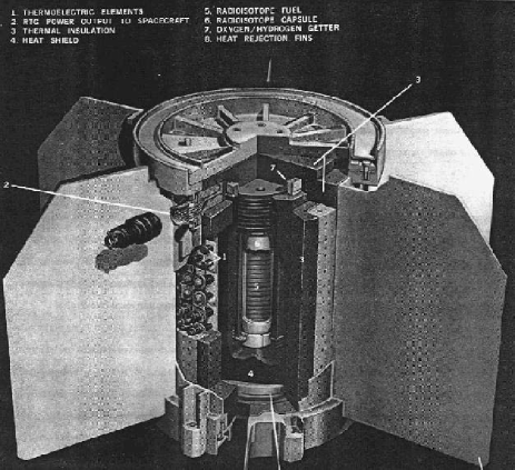
Figure 3: A design picture of the SNAP 19 RTGs. Note that for better heat radiation, this final design had much larger fins than those in the earlier spacecraft concept of Fig. 2.

Table 4: Thermal system and on-board power for Pioneers 10 and 11. The core of the system is four SNAP-19 RTGs (SNAP stands for Space Nuclear Auxiliary Power). These RTGs are fueled with Plutonium 238 that undergoes nuclear $\alpha$-decay via ₉₄Pu${}^{238}\rightarrow{}_{92}$U${}^{234}+{}_{2}$He⁴, with a half life of 87.74 yr. The efficiency of the relevant heat-to-electric power conversion is about 5 to 6%.

Power available:

$\triangleright$  before launch electric total 165 W (by 2001 $\approx 61$ W)

$\triangleright$   needs 100 W to power all systems ($\in$ 24.3 W science instruments)

Heat provided:

$\triangleright$   before launch thermal fuel total 2580 W (by 2001 $\approx 2050$ W)

$\triangleright$  electric heaters; 12 one-W RHUs

$\triangleright$   heat from the instruments (dissipation of 70 to 120 W)

Excess power/heat:      if electric power was $>$ 100 W $\Rightarrow$

$\triangleright$   thermally radiated into space by a shunt-resistor radiator, or

$\triangleright$   charge a battery in the equipment compartment

Thermal control:         to keep temperature within (0–90) F

$\triangleright$  thermo-responsive louvers: completely shut/fully open for 40 F/85 F

$\triangleright$  insulation: multi-layered aluminized mylar and kapton blankets

Problem 4.2. It has been argued that the anomalous acceleration is due to anisotropic heat reflection off of the back of the spacecraft high-gain antennas, the heat coming from the RTGs. Before launch, the four RTGs had a total thermal fuel inventory of 2580 W ($\approx 2050$ W in 2001). They produced a total electrical power of 165 W ($\approx 61$ W in 2001). (In Table 4 a description of the overall power system is given.) Thus, by 2002 approximatelly 2000 W of RTG heat still had to be dissipated. Because only $\approx 63$ W of directed power could have explained the anomaly, in principle, there was enough power to explain the anomaly.

The main bodies of the RTGs are cylinders and are grouped in two packages of two. Each package has two cylinders, end to end, extending away from the antenna. Each RTG has six fins separated by equal angles of $60^{\circ}$ that go radially out from the cylinder. The approximate dimensions for the RTGs are: the cylinder and fin lengths are 28.2 and 26.0 cm, the radius of the central RTG cylinder is 8.32 cm, and the RTG fin width as measured from the surface of the cylinder to the outer fin tip is 17.0 cm (see Fig. 3).

The RTGs are located at the end of booms, and rotate about the spacecraft in a plane that contains the approximate base of the antenna. From the closest axial center point of the RTGs, the antenna is seen nearly “edge on” (the longitudinal angular width is 24.5^∘). The total solid angle subtended is $\sim 1$–2% of $4\pi$ steradians. A more detailed calculation yields a value of 1.5%.

Estimate the contribution of the RTG heat reflecting off the spacecraft to the Pioneer anomaly. Can you explain the observed anomaly with this mechanism? Use the spacecraft geometry and the resultant RTG radiation pattern.

Solution 4.2. There are two reasons that preclude this mechanism. One is the spacecraft geometry. Even if we take the higher bound of 2% of 4$\pi$ steradians solid angle as the fraction of solid angle covered by the antenna, the equivalent fraction of the RTG heat could provide at most $\approx 40$ W. The second reason is the RTGs’ radiation pattern. Our estimate was based on the assumption that the RTGs are spherical black bodies, which they are not.

In fact, the fins are “edge on” to the antenna (the fins point perpendicular to the cylinder axes). The largest opening angle of the fins is seen only by the narrow angle parts of the antenna’s outer edges. If we ignore these edge effects, only $\approx 2.5$% of the surface area of the RTGs is facing the antenna, which is a factor of 10 less than that obtained from integrating the directional intensity from a hemisphere: $(\int^{\rm hemi}d\Omega\cos\theta)/(4\pi)=1/4$. Thus, we have only 4 W of directed power.

The force from 4 W of directed power suggests a systematic bias of $\approx 0.55\times 10^{-8}$ cm/s². If we add an uncertainty of the same size, we obtain a contribution from heat reflection of

$$a_{\rm hr}=(-0.55\pm 0.55)\times 10^{-8}\,\mbox{cm/s}^{2}.$$ (22)

If this mechanism were the cause, ultimately an unambiguous decrease in the size of $a_{P}$ should be observed, because the RTGs’ radioactively produced radiant heat is decreasing. As we noted, the heat produced is now about 80% of the original magnitude. In fact, we would expect a decrease of about $0.75\times 10^{-8}$ cm/s² in $a_{P}$ over the 11.5 year Pioneer 10 data interval if this mechanism were the origin of $a_{P}$.

Problem 4.3. Another suggestion related to the RTGs is the following: During the early parts of the missions, there might have been a differential change of the radiant emissivity of the solar-pointing sides of the RTGs with respect to the deep-space facing sides. Note that, especially closer in the Sun, the inner sides were subjected to the solar wind. On the other hand, the outer sides were sweeping through the solar system dust cloud. These two processes could result in different levels of degradation of the optical surfaces of the RTGs. In turn this degradation could result in asymmetric patterns of heat radiation away from the RTGs in the more/aft directions along the spin axis. Therefore, it can be argued that such an anisotropy may have caused the anomaly.

The six fins of each RTG, designed to provide the bulk of the heat rejection capacity, are fabricated of magnesium alloy.pioprd The metal is coated with two to three mils of zirconia in a sodium silicate binder to provide a high emissivity $(\approx 0.9)$ and low absorptivity $(\approx 0.2)$ (see Fig. 3).

Estimate the possible difference in the fore-and-aft emissivities of the RTGs needed to support this mechanism. Can this mechanism explain the observed anomaly? Discuss the significance of radioactive decay for this mechanism.

Solution 4.3. Depending on how symmetrically fore-and-aft they radiated, the relative fore-and-aft emissivity of the alloy would have had to have changed by $\approx 10$% to account for $a_{P}$. Given our knowledge of the solar wind and the interplanetary dust, this amount of a radiant change would be difficult to explain, even if it had the right sign.

To obtain a reasonable estimate of the uncertainty, consider if one side (fore or aft) of the RTGs has its emissivity changed by only 1% with respect to the other side. In a simple cylindrical model of the RTGs, with 2000 W power (only radial emission is assumed with no loss out of the sides), the ratio of the power emitted by the two sides would be $995/1005=0.99$, or a differential emission between the half cylinders of 10 W. Therefore, the fore/aft asymmetry toward the normal would be $10\,{\mathrm{W}}\times\frac{1}{\pi}\int_{0}^{\pi}d\phi\sin\phi\approx 6.37$ W.

A more sophisticated model of the fin structure starts off from ground zero to determine if we still obtain about the order of magnitude.pioprd Indeed we do, 6.12 W, which is the value we use in the following. (We refer the reader to Ref. pioprd, for this discussion, because the basic physics already has been discussed.)

If we take 6.12 W as the uncertainty from the differential emissivity of the RTGs, we obtain an acceleration uncertainty of

$$\sigma_{\rm de}=0.85\times 10^{-8}\,{\mathrm{cm/s}}^{2}.$$ (23)

Note that $10\,\sigma_{\rm de}$ almost equals our final result for $a_{P}$ (see Section VI). This correspondence is the origin of our previous statement that $\approx 10$% differential emissivity (in the correct direction) would be needed to explain $a_{P}$.

Finally, consider the significance of radioactive decay for this mechanism. The formal statistical error of the determination (before considering experimental systematics) was smallpioprd (see Sec. V). An example is a specific one-day “batch-sequential filtering”batch-seq value for $a_{P}$, averaged over the entire 11.5 year interval. This value was $a_{P}=(7.77\pm 0.16)\times 10^{-8}$ cm/s², where a batch-sequential error tends to be large. From radioactive decay, the value of $a_{P}$ should have decreased by $0.75\times 10^{-8}$ cm/s² over 11.5 years, which is five times the large batch sequential variance. Even more stringently, this bound is good for all radioactive heat sources. So, what if we were to argue that emissivity changes occurring before 1987 were the cause of the Pioneer effect? There still should have been a decrease in $a_{P}$ with time since then, which has not been observed.

Problem 4.4. Another possible on-board systematic error is from the expulsion of the He being created in the RTGs from the $\alpha$-decay of ²³⁸Pu.

The Pioneer RTGs were designed so that the He pressure is not totally contained within the Pioneer heat source over the life of the RTGs. Instead, the Pioneer heat source contains a pressure relief device that allows the generated He to vent out of the heat source and into the thermoelectric converter. The thermoelectric converter housing-to-power output receptacle interface is sealed with a viton O-ring. The O-ring allows the helium gas within the converter to be released by permeation into the space environment throughout the mission life of the Pioneer RTGs.

The actual fuel (see Fig. 3) is formed into a stack of disks within a container, each disk having a height of 0.212^′′ and a diameter of 2.145^′′. With 18 disks in each RTG and four RTGs per mission, the total volume of fuel is about 904 cm³. The fuel is a plutonium moly cermet and the amount of ²³⁸Pu in this fuel is about 5.8 kg. With a half life of 87.74 yr, the rate of He production (from plutonium $\alpha$-decay) is about 0.77 g/yr, assuming it all leaves the cermet and goes into the RTG chamber. To make this mechanism work, He leakage from the RTGs must be preferentially directed away from the Sun with a velocity large enough to cause the acceleration.

Can this mechanism explain the Pioneer anomaly? What is the largest effect possible with this mechanism? What is the uncertainty?

Solution 4.4. The operational temperature on the RTG surface at 433 K implies a helium velocity of 1.22 km/s. We use this value in the rocket equation,

$$a(t)=-v(t)\frac{d}{dt}[\ln M(t)].$$ (24)

We assume that the Pioneer mass corresponds to half of the fuel and that the gas is all unidirected and find a maximum bound on the possible acceleration of $1.16\times 10^{-8}$ cm/s². Thus, we can rule out helium permeating through the O-rings as the cause of $a_{P}$.

If we assume a single elastic reflection, we can estimate the acceleration biasbias in the direction away from the Sun. This estimate is $(3/4)\sin 30^{\circ}$ times the average of the heat momentum component parallel to the shortest distance to the RTG fin. By using this geometric information, we find the bias would be $0.31\times 10^{-8}$ cm/s². This bias effectively increases the value of the solution for $a_{P}$, which is too optimistic given all the complications of the real system. Therefore, we can take the systematic expulsion to be

$$a_{\rm He}=(0.15\pm 0.16)\times 10^{-8}\,\mathrm{cm/s}^{2}.$$ (25)

Problem 4.5. The effect of propulsive mass expulsion due to gas leakage has to be assessed. Although this effect is largely unpredictable, many spacecraft have experienced gas leaks producing accelerations on the order of $10^{-7}$ cm/s². Gas leaks generally behave differently after each maneuver. The leakage often decreases with time and becomes negligible.

Gas leaks can originate from Pioneer’s propulsion system, which is used for mid-course trajectory maneuvers, for spinning up or down the spacecraft, and for orientation of the spinning spacecraft. The Pioneers are equipped with three pairs of hydrazine thrusters, which are mounted on the circumference of the Earth-pointing high gain antenna. Each pair of thrusters forms a thruster cluster assembly with two nozzles aligned opposite to each other. For attitude control, two pairs of thrusters can be fired forward or aft and are used to precess the spinning antenna. The other pair of thrusters is aligned parallel to the rim of the antenna with nozzles oriented in co- and contra-rotation directions for spin/despin maneuvers.

During both observation intervals for the two Pioneers, there were no trajectory or spin/despin maneuvers. Thus, in this analysis we are mainly concerned with precession (that is, orientation or attitude control) maneuvers only. Because the valve seals in the thrusters can never be perfect, we ask if the leakages through the hydrazine thrusters could be the cause of the anomalous acceleration, $a_{P}$.

Consider the possible action of gas leaks originating from the spin/despin thruster cluster assembly. Each nozzle from this pair of thrusters is subject to a certain amount of gas leakage. But only a differential leakage from the two nozzles would produce an observable effect, causing the spacecraft to either spin down or up.

To obtain a gas leak uncertainty (and we emphasize uncertainty rather than “error” because there is no other evidence), we ask, “How large a differential force is needed to cause the spin down or spin up effects that are observed?” The answer depends on the moment of inertia about the spin axis, $I_{\rm z}\approx 588.3$ kg m², the antenna radius, $R=1.37$ m, and the observed spin down rates over three time intervals. In Ref. pioprd, the final effect was determined at the end by considering the spin-downs over the three time periods to be manifestations of errors that are uncorrelated and are normally distributed around zero mean. For simplicity, we include here the effect of this analysis in terms of an overall effective spin-down rate of $\ddot{\theta}=-0.0067$ rpm/yr.

Estimate the uncertainty in the value for the Pioneer anomaly from the possibility of undetected gas leaks.

Solution 4.5. If we use the information in Problem 4.5 and take the antenna radius, $R$, as the lever arm, we can calculate the differential force needed to torque the spin-rate change:

$$F_{\ddot{\theta}}=\frac{I_{\rm z}{\ddot{\theta}}}{R}=0.95\times 10^{-3}\,{\rm dyn}.$$ (26)

It is possible that a similar mechanism of undetected gas leakage could be responsible for the net differential force acting in the direction along the line of sight. In other words, what if there were some undetected gas leakage from the thrusters oriented along the spin axis of the spacecraft that is causing $a_{P}$? How large would this leakage have to be? A force of

$$F_{a_{P}}=ma_{P}=21.11\times 10^{-3}\,{\rm dyn}$$ (27)

($m=241$ kg) would be needed to produce our final unbiased value of $a_{P}$. Given the small amount of information, we conservatively take as our gas leak uncertainties the acceleration values that would be produced by differential forces equal to

$$F_{\rm gl}\approx\pm\sqrt{2}F_{\ddot{\theta}}=\pm 1.35\times 10^{-3}\,{\rm dyn}.$$ (28)

The argument for the result obtained in Eq. (28) is that we are accounting for the differential leakages from the two pairs of thrusters with their nozzles oriented along the line of sight direction. Equation (28) directly translates into the acceleration errors introduced by the leakage during the interval of Pioneer 10 data,

$$\sigma_{\rm gl}=\pm F_{\rm gl}/m=\pm 0.56\times 10^{-8}\,{\rm cm/s}^{2}.$$ (29)

At this point, we must conclude that the gas leak mechanism for explaining the anomalous acceleration is very unlikely, because it is difficult to understand why it would affect Pioneers 10 and 11 by the same amount. We also expect a gas leak would contribute to the anomalous acceleration, $a_{P}$, as a stochastic variable obeying a Poisson distribution. Instead, analyses of different data sets indicate that $a_{P}$ behaves as a constant bias rather than as a random variable.pioprd

Problem 4.6. There are two experimental results for the Pioneer anomaly from the two spacecraft: $7.84\times 10^{-8}$ cm/s² (Pioneer 10) and $8.55\times 10^{-8}$ cm/s² (Pioneer 11). The first result represents the entire 11.5 year data period for Pioneer 10; Pioneer 11’s result represents a 3.75 year data period.

The difference between the two craft could be due to different gas leakage. But it also could be due to heat emitted from the RTGs. In particular, the two sets of RTGs have had different histories and so might have different emissivities. Pioneer 11 spent more time in the inner solar system (absorbing radiation). Pioneer 10 has swept out more dust in deep space. Further, Pioneer 11 experienced about twice as much Jupiter/Saturn radiation as Pioneer 10. However, if the Pioneer effect is real, and not due to an extraneous systematic like heat, these numbers should be approximately equal.

Estimate the value for the Pioneer anomaly based on these two independent determinations. What is the uncertainty in this estimation?

Solution 4.6. We can calculate the time-weighted average of the experimental results from the two craft: $[(11.5)(7.84)+(3.75)(8.55)]/(15.25)=8.01$ in units of $10^{-8}$ cm/s². This result implies a bias of $b_{\rm 2,\,craft}=0.17\times 10^{-8}$ cm/s² with respect to the Pioneer 10 experimental result $a_{P({\rm exp})}$ (see Eq. (35) below). In addition, we can take this number to be a measure of the uncertainty from the separate spacecraft measurements, so the overall quantitative measure is

$$a_{\rm 2,\,craft} = b_{\rm 2,\,craft}\pm\sigma_{\rm 2,\,craft}$$ (30)

$$= (0.17\pm 0.17)\times 10^{-8}\,\mathrm{cm/s}^{2}.$$

V Sources of computational errors

Given the very large number of observations for the same spacecraft, the error contribution from observational noise is very small and not a meaningful measure of uncertainty. It is therefore necessary to consider several other effects in order to assign realistic errors. The first consideration is the statistical and numerical stability of the calculations. Then there is the cumulative influence of all program modeling errors and data editing decisions. Besides these factors, there are errors that may be attributed to the specific hardware used to run the orbit determination computer codes, together with the algorithms and statistical methods used to obtain the solution. These factors have been included in the summary of the biases and uncertainties given in Table 5. The largest contributor in this category, and the question we will discuss here, is the reason for and significance of a periodic term that appears in the data.

Table 5: Error budget: A summary of biases and uncertainties.

Item	Description of error budget constituents	Bias	Uncertainty
		$10^{-8}$ cm/s2	$10^{-8}$ cm/s2
1.	Sources of acceleration noise external to the craft
	(a) Solar radiation pressure	$+0.03$	$\pm 0.01$
	(b) Solar wind		$\pm<10^{-3}$
	(c) Solar corona		$\pm 0.02$
	(d) Electromagnetic Lorentz forces		$\pm<10^{-4}$
	(e) Phase stability and clocks		$\pm<0.001$
2.	On-board sources of acceleration noise
	(a) Radio beam reaction force	$+1.10$	$\pm 0.10$
	(b) RTG heat reflected off the craft	$-0.55$	$\pm 0.55$
	(c) Differential emissivity of the RTGs		$\pm 0.85$
	(d) Non-isotropic radiative cooling of the spacecraft		$\pm 0.48$
	(e) Expelled Helium produced within the RTGs	$+0.15$	$\pm 0.16$
	(f) Gas leakage		$\pm 0.56$
	(g) Variation between spacecraft determinations	$+0.17$	$\pm 0.17$
3.	Sources of computational errors
	(a) Accuracy of consistency/model tests		$\pm 0.13$
	(b) Annual term		$\pm 0.32$
	(c) Other important effects		$\pm 0.04$
	Estimate of total bias/error	$+0.90$	$\pm 1.33$

Problem 5.1. In addition to the constant anomalous acceleration term, an annual sinusoid has been reported.pioprd The peaks of the sinusoid occur when the Earth is exactly on the opposite side of the Sun from the craft, where the Doppler noise is at a maximum. The amplitude of this oscillatory term by the end of the data interval was $\approx 0.22\times 10^{-8}$ cm/s². The integral of a sine wave in the acceleration, with angular velocity $\omega$ and amplitude $a_{0},$ yields the following first-order Doppler amplitude, in the fractional frequency change accumulated over the round-trip travel time of the radio-signal:

$$\frac{\Delta\nu}{\nu}=\frac{2a_{0}}{c\omega}.$$ (31)

The resulting Doppler amplitude from the sine wave with amplitude of $a_{0}=0.22\times 10^{-8}$ cm/s² and annual angular velocity $\omega=2\times 10^{-7}$ rad/s is $\Delta\nu/\nu=7.3\times 10^{-13}$. At the Pioneer downlink S-band carrier frequency of $\approx 2.29$ GHz, the corresponding Doppler amplitude is 0.002 Hz, that is, 0.11 mm/s.

A four-parameter, nonlinear, weighted, least-squares fit to the annual sine wave was found with the amplitude $v_{\rm at}=(0.1053\pm 0.0107)$ mm/s, phase $=(-5.3^{\circ}\pm 7.2^{\circ}$), angular velocity $\omega_{\rm at}=(0.0177\pm 0.0001$) rad/day, and bias $=(0.0720\pm 0.0082$) mm/s. Standard data weighting procedurespioprd yield post-fit weighted rms residuals of $\sigma_{T}=0.1$ mm/s (the Doppler error averaged over the data interval $T$).

The amplitude, $v_{\rm at}$, and angular velocity, $\omega_{\rm at}$, of the annual term result in a small acceleration amplitude of $a_{\rm at}=v_{\rm at}\omega_{\rm at}=(0.215\pm 0.022)\times 10^{-8}$ cm/s². The cause is most likely due to errors in the navigation programs’ determinations of the direction of the spacecraft’s orbital inclination to the ecliptic. Estimate the annual contribution to the error budget for $a_{P}$.

Solution 5.1. First observe that the standard errors for the radial velocity, $v_{r}$, and acceleration, $a_{r}$, are essentially what would be expected for a linear regression. The caveat is that they are scaled by the root sum of squares of the Doppler error and unmodeled sinusoidal errors, rather than just the Doppler error. Furthermore, because the error is systematic, it is unrealistic to assume that the errors for $v_{r}$ and $a_{r}$ can be reduced by a factor 1/$\sqrt{N}$, where $N$ is the number of data points. Instead, if we average their correlation matrix over the data interval, $T$, we obtain the estimated systematic error of

$$\sigma_{a_{r}}^{2}=\frac{12}{T^{2}}\,\sigma_{v_{r}}^{2}=\frac{12}{T^{2}}(\sigma_{T}^{2}+\sigma_{v_{\rm at}}^{2}),$$ (32)

where $\sigma_{T}=0.1$ mm/s is the Doppler error averaged over $T$ (not the standard error of a single Doppler measurement), and $\sigma_{v_{\rm at}}$ is equal to the amplitude of the unmodeled annual sine wave divided by $\sqrt{2}$. The resulting root sum of squares error in the radial velocity determination is about $\sigma_{v_{r}}=(\sigma_{T}^{2}+\sigma_{v_{\rm at}}^{2})^{1/2}=0.15$ mm/s for both Pioneer 10 and 11. Our values of $a_{P}$ were determined over time intervals of longer than a year. At the same time, to detect an annual signature in the residuals, we need at least half of the Earth’s orbit to be complete. Therefore, with $T=1/2$ yr, Eq. (32) results in an acceleration error of

$$\sigma_{{\rm a_{r}}}=\frac{0.50\,{\rm mm/s}}{T}=0.32\times 10^{-8}\,{\mathrm{cm/s}}^{2}.$$ (33)

This number is assumed to be the systematic error from the annual term.

VI Summary of ERRORs AND FINAL RESULT

The tests discussed in the preceding sections have considered various potential sources of systematic error. The results are summarized in Table 5. The only major source of uncertainty not discussed here is the non-isotropic radiative cooling of the spacecraft.pioprd ; mpla Other more minor effects are discussed in Ref. pioprd, . Table 5 summarizes the systematic errors affecting the measured anomalous signal, the “error budget” of the anomaly. It is useful for evaluating the accuracy of the solution for $a_{P}$ and for guiding possible future efforts with other spacecraft.

Finally, there is the intractable mathematical problem of how to handle combined experimental systematic and computational errors. In the end it was decided to treat them all in a least squares uncorrelated manner.pioprd

Problem 6.1. The first column in Table 5 gives the bias, $b_{P}$, and the second gives the uncertainty, $\pm\sigma_{P}$. The constituents of the error budget are listed in three categories: systematic errors generated external to the spacecraft; on-board generated systematic errors, and computational errors. Our final result will be an average

$$a_{P}=a_{P({\rm exp)}}+b_{P}\pm\sigma_{P},$$ (34)

where

$$a_{P({\rm exp)}}=(7.84\pm 0.01)\times 10^{-8}\,{\mathrm{cm/s}}^{2}$$ (35)

is our formal solution for the Pioneer anomaly that was obtained with the available data set.pioprd

Discuss the contributions of various effects to the total error budget and determine the final value for the Pioneer anomaly, $a_{P}$.

Solution 6.1. The least significant factors of our error budget are in the first group of effects, those external to the spacecraft. From Table 5 we see that some are near the limit of contributing, and in total they are insignificant.

The on-board generated systematics are the largest contributors to the total. All the important constituents are listed in the second group of effects in Table 5. Among these effects, the radio beam reaction force produces the largest bias, $1.10\times 10^{-8}$ cm/s², and makes the Pioneer effect larger. The largest bias/uncertainty is from RTG heat reflecting off the spacecraft. The effect is as large as $(-0.55\pm 0.55)\times 10^{-8}$ cm/s². Large uncertainties also come from differential emissivity of the RTGs, radiative cooling, and gas leaks, $\pm 0.85$, $\pm 0.48$, and $\pm 0.56$, respectively, $\times 10^{-8}$ cm/s².

The computational errors are listed in the third group of Table 5. We obtain $b_{P}\pm\sigma_{P}=0.90\times 10^{-8}$ cm/s² and $\sigma_{P}=1.33\times 10^{-8}$ cm/s². Therefore, from Eq. (34) the final value for $a_{P}$ is

$$a_{P}=(8.74\pm 1.33)\times 10^{-8}\,\mbox{cm/s}^{2}.$$ (36)

The effect is clearly significant and remains to be explained.

Appendix A Allan deviation

To achieve the highest accuracy, the Doppler frequency shift of the carrier wave is referenced to ground-based atomic frequency standards. The observable is the fractional frequency shift of the stable and coherent two-way radio signal (Earth-spacecraft-Earth)

$$y(t)=\frac{\nu_{\rm r}(t)-\nu_{\rm t}}{\nu_{\rm t}}=\frac{2}{c}\frac{dL}{dt},$$ (37)

where $\nu_{\rm r}$ and $\nu_{\rm t}$ are, respectively, the transmitted and received frequencies, $t$ is the receiving time, and $2L$ is the overall optical distance (including diffraction effects) traversed by the photon in both directions.

The received signal is compared with the expected measurement noise in $y$, given by Eq. (37). The quality of such a measurement is characterized by its Allan deviation, which defined as

$$\sigma_{y}(\tau)=\sqrt{\frac{1}{2}\langle(\bar{y}_{i+1}(\tau)-\bar{y}_{i}(\tau))^{2}\rangle},$$ (38)

where ${\bar{y}}_{i}=\frac{1}{\tau}\int_{t_{i}}^{t_{i}+\tau}y(t)dt$. The Allan deviation is the most widely used figure of merit for the characterization of frequency in this context.

For advanced planetary missions such as Cassini, equipped with multi-frequency links in the X- and Ka-bands, Allan deviations reach the level of $\sigma_{y}\approx 10^{-14}$ for averaging times between $10^{3}$ and $10^{4}$ s. The Pioneer spacecraft were equipped with S-band Doppler communication systems for which Allan deviations were usually the order ofl of $1.3\times 10^{-12}$ and $1.0\times 10^{-12}$, respectively, for $10^{3}$ s Doppler integration times.

References

- (1) J. D. Anderson, P. A. Laing, E. L. Lau, A. S. Liu, M. M. Nieto, and S. G. Turyshev, “Indication, from Pioneer 10/11, Galileo, and Ulysses data, of an apparent anomalous, weak, long-range acceleration,” Phys. Rev. Lett. 81, 2858–2861 (1998), gr-qc/9808081.
- (2) J. D. Anderson, P. A. Laing, E. L. Lau, A. S. Liu, M. M. Nieto and S. G. Turyshev, “Study of the Anomalous Acceleration of Pioneer 10 and 11,” Phys. Rev. D 65, 082004/1–50 (2002), gr-qc/0104064.
- (3) To be precise, the data analyzed in Ref. pioprd, was taken between 3 January 1987 and 22 July 1998 for Pioneer 10 (when the craft was 40 AU to 70.5 AU distant from the Sun), and that from Pioneer 11 was obtained between 5 January 1987 and 1 October 1990 (22.4 to 31.7 AU).
- (4) E. M. Murphy, “Prosaic explanation for the anomalous acceleration seen in distant spacecraft,” Phys. Rev. Lett. 83, 1890 (1999), gr-qc/9810015.
- (5) J. I. Katz, “Comment on ‘Indication, from Pioneer 10/11, Galileo, and Ulysses data, of an apparent anomalous, weak, long-range acceleration’,” Phys. Rev. Lett. 83, 1892 (1999), gr-qc/9809070.
- (6) L. K. Scheffer, “Conventional forces can explain the anomalous acceleration of Pioneer 10,” Phys. Rev. D 67, 084021/1–11 (2003), gr-qc/0107092.
- (7) J. D. Anderson, P. A. Laing, E. L. Lau, A. S. Liu, M. M. Nieto, and S. G. Turyshev, “Anderson et al. reply,” Phys. Rev. Lett. 83, 1891 (1999), gr-qc/9906113.
- (8) J. D. Anderson, P. A. Laing, E. L. Lau, A. S. Liu, M. M. Nieto, and S. G. Turyshev, “Anderson et al. reply,” Phys. Rev. Lett. 83, 1893 (1999), gr-qc/9906112.
- (9) J. D. Anderson, E. L. Lau, S. G. Turyshev, P. A. Laing, and M. M. Nieto, “The search for a standard explanation of the Pioneer anomaly,” Mod. Phys. Lett. A 17, 875–885 (2002), gr-qc/0107022.
- (10) C. B. Markwardt, “Independent confirmation of the Pioneer 10 anomalous acceleration,” gr-qc/0208046.
- (11) M. M. Nieto and S. G. Turyshev, “Finding the origin of the Pioneer anomaly,” Class. Quant. Grav. 21, 4005–4023 (2004), gr-qc/0308017.
- (12) J. D. Anderson, S. G. Turyshev, and M. M. Nieto, “A mission to test the Pioneer anomaly,” Int. J. Mod. Phys. D 11, 1545–1551 (2002), gr-qc/0205059.
- (13) S. G. Turyshev, M. M. Nieto, and J. D. Anderson,“Lessons learned from the Pioneers 10/11 for a mission to test the Pioneer anomaly,” Adv. Space Res., Proc. 35th COSPAR Scientific Assembly (Paris, 2004), to be published, gr-qc/0409117.
- (14) M. M. Nieto, S. G. Turyshev, and J. D. Anderson, “The Pioneer anomaly: The data, its meaning, and a future test,” in Proceedings of the 2nd Mexican Meeting on Mathematical and Experimental Physics, edited by A. Macías, C. Lämmerzahl, and D. Nuñez (American Institute of Physics, NY, 2005), pp. 113-128, gr-qc/0411077.
- (15) S. G. Turyshev, M. M. Nieto, and J. D. Anderson, “A route to understanding of the Pioneer anomaly,” in Proceedings of the XXII Texas Symposium on Relativistic Astrophysics, Stanford University, December 13–17, 2004, edited by P. Chen, E. Bloom, G. Madejski, and V. Petrosian. SLAC-R-752, Stanford e-Conf #C041213, paper #0310, eprint: <http://www.slac.stanford.edu/econf/C041213/>, gr-qc/0503021.
- (16) M.-T. Jaekel and S. Reynaud, “Gravity tests in the solar system and the Pioneer anomaly,” Mod. Phys. Lett. A, 20, 1047-1055 (2005), gr-qc/0410148.
- (17) R. H. Sanders, “A tensor-vector-scalar framework for modified dynamics and cosmic dark matter,” astro-ph/0502222.
- (18) J. W. Moffat, “Scalar-tensor-vector gravity theory,” gr-qc/0506021.
- (19) A. F. Ranada, “The Pioneer anomaly as acceleration of the clocks,” Found. Phys. 34, 1955–1971 (2005), gr-qc/0410084.
- (20) R. Foot and R. R. Volkas, “A mirror world explanation for the Pioneer spacecraft anomalies?,” Phys. Lett. B 517, 13–17 (2001), hep-ph/0108051.
- (21) G. L. Tyler, J. P. Brenkle, T. A. Komarek, and A. I. Zygielbaum, “The Viking Solar Corona experiment,” J. Geophys. Res. 82, 4335–4340 (1977).
- (22) D. O. Muhleman, P. B. Esposito, and J. D. Anderson, “The electron density profile of the outer corona and the interplanetary medium from Mariner-6 and Mariner-7 time-delay measurements,” Astrophys. J. 211, 943–957 (1977).
- (23) D. O. Muhleman and J. D. Anderson, “Solar wind electron densities from Viking dual-frequency radio measurements,” Astrophys. J. 247, 1093–1101 (1981).
- (24) S. G. Turyshev, B-G Andersson, “The 550 AU Mission: A Critical Discussion,” Mon. Not. Roy. Astron. Soc. 341, 577–582 (2003), gr-qc/0205126.
- (25) For a discussion of spacecraft charging, see <http:// www.eas.asu.edu/~holbert/eee460/spc-chrg.html>. However, the magnetic field strength in the outer solar system is on the order of Gauss.
- (26) G. W. Null, “Gravity field of Jupiter and its satellites from Pioneer 10 and Pioneer 11 tracking data,” Astron. J. 81, 1153–1161 (1976).
- (27) The NASA Deep Space Network (DSN) is an international network of antennae spread nearly equidistantly around the Earth with one complex being situated in Goldstone, California, the second one near Canberra, Australia, and the third one near Madrid, Spain.pioprd For more details, see <http://deepspace.jpl.nasa.gov/dsn/>.
- (28) To determine the state of the spacecraft at any given time, the Jet Propulsion Laboratory’s orbit determination program uses a batch-sequential filtering and smoothing algorithm with process noise.pioprd For this algorithm, any small anomalous forces may be treated as stochastic parameters affecting the spacecraft trajectory. As such, these parameters are also responsible for the stochastic noise in the observational data. To better characterize these noise sources, the data interval is split into a number of constant or variable size intervals, called “batches,” and assumptions are made for statistical properties of these noise factors. The mean values and the second moments of the unknown parameters are estimated within the batch. In batch sequential filtering, the reference trajectory is updated after each batch to reflect the best estimate of the true trajectory. (For more details consult Ref. pioprd, and also references therein.)
- (29) We use the symbol to identify biases in the measured value of the Pioneer anomaly produced by various sources of acceleration noise. The uncertainly in the contribution of these noise sources to the anomalous acceleration is conventionally denoted by . See an example of this usage in Eq. (21).