Additive-multiplicative stochastic models of financial mean-reverting processes

Abstract

We investigate a generalized stochastic model with the property known as mean reversion, that is, the tendency to relax towards a historical reference level. Besides this property, the dynamics is driven by multiplicative and additive Wiener processes. While the former is modulated by the internal behavior of the system, the latter is purely exogenous. We focus on the stochastic dynamics of volatilities, but our model may also be suitable for other financial random variables exhibiting the mean reversion property. The generalized model contains, as particular cases, many early approaches in the literature of volatilities or, more generally, of mean-reverting financial processes. We analyze the long-time probability density function associated to the model defined through a Itô-Langevin equation. We obtain a rich spectrum of shapes for the probability function according to the model parameters. We show that additive-multiplicative processes provide realistic models to describe empirical distributions, for the whole range of data.

I Introduction

Accurate statistical description of the stochastic dynamics of stock prices is fundamental to investment, option pricing and risk management. In particular, a relevant quantity is the volatility of price time seriesvolatility , that quantifies the propensity of the market to fluctuate. Since volatility represents a measure of the risk associated to the fluctuating dynamics of prices, it is crucial to develop suitable models to predict its complex intermittent behavior. There is empirical evidence that it fluctuates following a stochastic dynamics subjacent to that of prices, whose dynamics, in turn, depends on the time evolving volatility. Many approaches are based on that assumptionprices , although others propose the existence of a reciprocal feedback between both processesleverage .

Our approach builds on the development of a simple Langevin equation to characterize the stochastic process of volatility. The equation provides an unifying description that generalizes widely discussed models in the literature. We analyze the shape of the long-time probability density function (PDF) associated to the stochastic differential equation that characterizes each particular case of the generalized model. Most previous results focus on the tails of the PDFs. In fact, for stochastic variables, such as volatilities presenting fat-tailed PDFsliu ; volat1 , it is specially important to reproduce extreme events in a realistic model. Now we go a step further and aim to predict the PDFs in the whole range of events.

One of the main features observed in the dynamics of some financial variables, such as volatilities, stock volumes or interest rates, is their tendency to permanently relax, towards a reference level $\theta$, a property known as mean reversion. Another feature is the multiplicative market processing of random news, whose strength becomes modulated by a function of the stochastic variable itself. These two properties are modeled by means of a nonlinear mean-reverting force and nonlinear multiplicative noise. They are discussed in detail in Sect. II.

In Sect. III, we discuss the shapes of the PDFs that such family of models yields. Despite being of a general form, they give rise to PDFs that, decay exponentially fast, either above the mode, below it, or both, in disagreement with empirical observations. For instance, log-normal behavior has been reported for volatility computed from global data of S&P500liu , at intermediate values. However, at high values, a power-law behavior, with exponent outside the stable Lévy range, was observed. The same analysis performed for individual companiesliu yields also power-law tails. But in that case, the results show a variation slower than log-normal below the mode, suggesting a power-law also in the limit of small values. The volatility of capitalized stocks traded in US equity markets exhibits similar featuresmicciche . Other variables with mean-reversion, such as volume of transactions (number of trades) present akin distributions. Power-law tails out of the Lévy range have been reported for the PDFs of normalized NYSE stock volumesvolumes . More recently, studies of normalized volumes, performed over high resolution data (1-3 minutes) of NYSE and NASDAQvol1 (see also vol2 ), display PDFs with power-law behavior both at large and small values. We will show that the class of multiplicative processes considered in Sect. III, although general enough, is not able to reproduce, for any value of its parameters, these empirical PDFs in the whole range.

In a realistic model, we must deal with various sources of fluctuations acting upon the collective variable. Then, we propose to include a component that is lacking to suitably model many real processes, that is the presence of fluctuations that act additively, besides the multiplicative noise already taken into account. The latter originates from the internal correlated behavior of the market, representing a sort of endogenous feed-back effect, while additive noise concerns fluctuations of purely external origin or random speculative trading. Then, in Sect. IV, we present a further generalization that consists in incorporating an independent additive source of noise. Depending on the parameters of the process, the additive or multiplicative contributions will play the dominant role. This gives rise to a rich spectrum of PDF shapes, in particular, a subclass with two-fold power-law behavior, both above and below the mode, providing a general realistic framework for describing the shape of empirical distributions. A comparison with experimental results is presented in Sect. V. Finally, Sect. VI contains the main conclusions and general remarks.

II Mean reversion and multiplicative fluctuations

The reversion to the mean is one of the basic ingredients to describe the dynamics of several stochastic variables of interest in economy. It is fundamental since it concerns the behavior around a central value $\theta$ and reflects the global market response to deviations from a consensus or equilibrium level. It depends on monetary unit, market size, degree of risk aversion, etc., hence, it is characteristic of each market. The aversion to deviations from the mean needs not be linear, specially when large deviations are involved. Similarly, a nonlinear mechanism due to the cooperative behavior of traders, rules the way the market modulates the amplitude of fluctuations (mainly external) giving rise to innovations.

We consider the general class of stochastic differential equations given by

$${\rm d}x\;=\;-\gamma[x-\theta]x^{r-1}{\rm d}t+\mu x^{s}{\rm d}w\;,$$ (1)

where, $\theta,\gamma,\mu>0$, $r,s\in\mathbb{R}$, and $w$ is a Wiener process, such that $\langle{\rm d}w\rangle=0$ and $\langle({\rm d}w)^{2}\rangle=2{\rm d}t$. The definition of the stochastic process is completed by the Itô prescription. This class generalizes well-known models employed to describe the dynamics of mean-reverting financial variablesjuros . In particular, some traditional processes for modeling volatilities or, mainly, squared volatilities are the Hull-White ($r=1,s=1$)hw and the Heston ($r=1,s=1/2$)heston models, the latter also known either as Cox-Ingersoll-Rosscir or Feller processfeller . The arithmetic ($r=1,s=0$) and geometric ($r=2,s=1$) Ornstein-Ulhenbeck processes are particular cases too. Moreover, several other models employed in the literature of volatilities are related to this classothers ; micciche .

Different values of $r$ in Eq. (1) represent different possible relaxation mechanisms of amplitude $\gamma$, determined, amongst other factors, by constraints, flux of information, stock liquidity and risk aversion, which are particular of a given market. Notice that the restoring force in Eq. (1) corresponds to a confining potential, with minimum at $\theta$, for all $r\in\mathbb{R}$. The larger $r$, the more attractive the potential for large $x$, but the less attractive for vanishing $x$. Similarly, different values of $s$ specify the market informational connectivity, which conditions the degree of coherent multiplicative behavior. Models in the literature typically set $s\geq 0$, meaning that the effective amplitude of fluctuations increases with $x$. Negative $s$ makes multiplicative fluctuations grow with decreasing $x$, thus it mainly reflects a cooperative reaction to quiescence. Although it does not seem to reflect a realistic steady state of the market, it may occur as a transient, driven by speculative trading.

The two mechanisms are complementary. If $r<0$ the restoring force decreases for increasing $x$ above the reference level, in particular, for $r<-1$, the force tends to zero in the limit of large $x$. Thus, decreasing $r$ represents markets that, become less able to recover the reference level by means of the deterministic tendency alone. However, a strong multiplicative response to large fluctuations (positive $s$) could still compensate that inability and restore the market historical level. Concerning the response to small values, the restoring force diverges at the origin if $r<1$, while for $r>1$, it vanishes at $x=0$, meaning that this point becomes an unstable equilibrium state. This corresponds to a market indifferent to low levels of trading activity. Again, this effect can be balanced by the multiplicative contribution (with a small value of parameter $s$).

In early works, only very particular values of $(r,s)$ have been considered. However, this may be sometimes owed more to reasons of mathematical solvability, than to econophysical ones. Following the above discussion, $(r,s)$ may be non-universal, depending on the particular nature of a market or its agents. Therefore, we will not discard any possibility a priori.

III Generalized multiplicative process with mean reversion

We consider the simple class of stochastic multiplicative differential equations given by Eq. (1), that generalizes many processes usually found in the literature of volatilities. We investigate, in this Section, the long-time PDFs that this class of processes yields. The Fokker-Planck equation associated to Eq. (1), following standard methodsbooks , is

$$\partial_{t}\rho=\gamma\partial_{x}([x-\theta]x^{r-1}\rho)+\mu^{2}\partial^{2}_{xx}[x^{2s}\rho]\;.$$ (2)

Its long-term solution is relevant in connection to the assumption that the process can be treated as quasi-stationary. In that case the PDF obtained from an actual data series will coincide with the stationary solution. Considering reflecting boundary conditions at $x=0$ and $x\to\infty$books , the steady state solution of Eq. (2) reads:

$$\rho(x)=\frac{\rho_{o}}{x^{2s}}\exp\left(-\gamma_{\mu}\Bigl{[}\frac{x^{p+1}}{p+1}-\theta\frac{x^{p}}{p}\Bigr{]}\right),$$ (3)

with $p\equiv r-2s\neq 0,-1$, where $\rho_{o}$ is a normalization constant and $\gamma_{\mu}\equiv\gamma/\mu^{2}$ an effective restoring amplitude, such that $\gamma$ (a parameter associated to order) becomes reduced by the amplitude of multiplicative noise (associated to disorder).

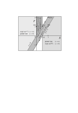
Figure 1: Diagram of the asymptotic behavior of the PDF given by Eq. (3), in ($s,r$)-plane. Unshadowed regions and dotted borders identify regions excluded by the normalization condition. At the positive $r$-axis, the PDF is finite at the origin. Tilted lines denote the marginal cases $r=2s$ ($p=0$), with pure exponential tail and power-law growth at the origin, and $r=2s-1$ ($p=-1$), with power-law tail and exponential of $1/x$ growth at the origin (the threshold points of these lines have coordinates $([1+\gamma_{\mu}\theta]/2,0)$ and $([1-\gamma_{\mu}]/2,0)$, respectively). Parameter $a>0$, in the exponential formulas, as well as the power-law exponents, depend on model parameters. Symbols correspond to the special processes: Hull-White (HW), Heston (H), Ornstein-Ulhenbeck (OU) and geometric OU (GOU).

The class of processes described by Eq. (3) thus generically yields asymptotic exponential-like behaviors for small or/and large values. As soon as $p+1>0$, a stretched exponential decay is obtained for large enough $x$, such that the argument of the exponential is proportional to $-x^{p+1}$. If $p<0$, a stretched exponential of the inverse argument ($-1/x^{|p|}$) is obtained for vanishing $x$. Therefore, for $p\in(-1,0)$, the PDF presents dominant exponential-like behavior both for low and large values, without any restriction on the value of $s$. Outside that interval, the power law $x^{-2s}$ in (3) asymptotically dominates, for either small (if $p>0$) or large (if $p<-1$) argument. Then, normalization in $[0,\infty)$ restricts the possible values of $s$ according to: $s<1/2$ (if $p>0$), $x>1/2$ (if $p<-1$).

In the marginal cases, Eq. (3) explicitly is:

I: For $p\equiv r-2s=-1,$

$$\rho(x)=\frac{\rho_{o}}{x^{2s+\gamma_{\mu}}}\;\exp(-\gamma_{\mu}\theta/x)\;,$$ (4)

with $2s>1-\gamma_{\mu}$ for nomalizability.

II: For $p\equiv r-2s=0$,

$$\rho(x)=\rho_{o}x^{\gamma_{\mu}\theta-2s}\exp(-\gamma_{\mu}x)\;,$$ (5)

with $2s<\gamma_{\mu}\theta+1$ for normalization, but $2s<\gamma_{\mu}\theta$ to avoid the divergence at the origin.

Fig. 1 displays the possible PDF asymptotic shapes in $(s,r)$ space. Notice that the $s=0$ axis gives the solution for mean-reverting models with purely additive fluctuations. Let us analyze some special cases. In the trivial case $(s,r)=(0,1)$, corresponding to the Ornstein-Ulhenbeck process books

$${\rm d}x\;=\;-\gamma[x-\theta]{\rm d}t+\mu{\rm d}z\;,$$ (6)

the noisy contribution becomes additive and the stationary PDF is Gaussian (truncated at $x=0$).

Although we are dealing with $\theta>0$, it is worth of mention the case $(\theta,s,r)=(0,1,1)$, corresponding to the geometric Brownian process, that leads to the log-normal distribution.

For type I ($r=2s-1$), notice that the PDF decays as a power law, for large $x$, and goes to zero faster than power law, for vanishing $x$. The power-law exponent is controlled by $s$ and $\gamma_{\mu}$, that is, all the model parameters, except $\theta$ are involved. In the particular case $r=s=1$, one recovers the Hull-White processhw

$${\rm d}x\;=\;-\gamma[x-\theta]{\rm d}t+\mu x{\rm d}z\;.$$ (7)

In case II ($r=2s$), observe that the PDF has opposite behavior: it increases at the origin as a power law and decays exponentially for large $x$. All the model parameters, including $\theta$ are buried in the power-law exponent. In particular, if $r=2s=1$, one gets the Heston modelheston

$${\rm d}x\;=\;-\gamma[x-\theta]{\rm d}t+\mu\sqrt{x}{\rm d}z\;.$$ (8)

If $r=2s=2$, the geometric Ornstein-Uhlenbeck process is obtained

$${\rm d}x\;=\;-\gamma[x-\theta]x{\rm d}t+\mu x{\rm d}z\;.$$ (9)

Diverse other models proposed in the literature can also be thought as particular instances of our generalized model. For example, the one proposed by Micciché et al. micciche is in correspondence with the Hull-White model (7), with $x$ representing volatility $v$, whereas in the latter $x\equiv v^{2}$. Also a family of multiplicative models, studied before in the context of a wide spectrum of physical processesschenzle , belongs to the class here considered, through the transformation $x\to x^{\beta}$.

Summarizing, from Eqs. (3)-(5), in general, the asymptotic behaviors below and above the mode are tied, such that, in a log-log scale, if one flattens the other changes rapidly. This explains why models of this class fail to describe empirical volatilities in the whole range of observed data, even under the transformation $v^{2}\mapsto v$.

IV Generalized model with additive-multiplicative structure

We analyze in this section, processes that take into account the presence of some additional source of noise. Previous worksmulti1 ; multi2 ; multi3 show that additive-multiplicative stochastic processes constitute an ubiquitous mechanism leading to fat-tailed distributions and correlated sequences. This extra noise represents a quite realistic feature, since, besides noise modulated by the market, other fluctuations may act directly, additively. From the stream of news, represented by a noisy signal, some are amplified or reduced by cooperative actions, others incorporated unaltered. Related ideas has been discussed in Ref. sornette . Also, a model of financial markets that leads to additive-linear-multiplicative processes has been recently proposedspins , where the noises are identified with the fluctuating environment and fluctuating interaction network, respectively. In general, the two white noises are considered uncorrelated. However, they may even correspond to identical time-series as soon as they are shifted with a time lag greater than the correlation time. In such case, the endogenous noise is expected to act with a delay due to its very nature of feedback process, whereas, the additive noise is incorporated immediately, free of signal processing.

By including purely exogenous fluctuations, in the process defined by Eq. (1), we obtain the following Itô-Langevin equation (ILE)

$${\rm d}x\;=\;-\gamma[x-\theta]x^{r-1}{\rm d}t+\mu x^{s}{\rm d}w+\alpha{\rm d}z\;,$$ (10)

where $w,z$ are two independent standard Wiener processes, defined as above, and $\mu,\alpha$ their respective amplitudes. The corresponding Fokker-Planck equation reads

$$\partial_{t}\rho=\gamma\partial_{x}([x-\theta]x^{r-1}\rho)+\partial_{xx}([\mu^{2}x^{2s}+\alpha^{2}]\rho)\;.$$ (11)

Its steady state solution with reflecting boundary conditions is

$$\rho(x)=\frac{\rho_{o}}{1+\lambda^{2}x^{2s}}\exp[-\gamma_{\alpha}\int^{x}\frac{y^{r-1}(y-\theta)}{1+\lambda^{2}y^{2s}}{\rm d}y]\;,$$ (12)

with $\rho_{o}$ a normalization constant, $\gamma_{\alpha}\equiv\gamma/\alpha^{2}$, $\lambda^{2}\equiv(\mu/\alpha)^{2}\equiv\gamma_{\alpha}/\gamma_{\mu}$. In most cases the integral can be written in terms of hypergeometric functions ${}_{2}F_{1}$abram , through

$$\int^{x}\frac{y^{\beta-1}}{1+\lambda^{2}y^{2s}}{\rm d}y\equiv\frac{\beta}{x^{\beta}}\,_{2}F_{1}(c,1,c+1,-\lambda^{2}x^{2s})$$ (13)

with $c\equiv\beta/(2s)\neq-1,-2,\ldots$, whereas, in the marginal case $\beta=0$, we will use

$$\int^{x}\frac{y^{-1}}{1+\lambda^{2}y^{2s}}{\rm d}y\;\equiv\;\ln x\,-\,\ln(1+\lambda^{2}x^{2s})/(2s).$$ (14)

By means of these definitions and their asymptotic formulasabram ; formula , we obtain the possible PDF shapes, in $(s,r)$-space, as schematized in Fig. 2. The marginal cases $r=0$ and $r=-1$ will be considered latter. In general, sufficiently large positive $s$ is required in order to yield power-law tails, otherwise, stretched exponential tails prevail, as for the processes considered in Sect. III. The additive noise does not add new domains with power-law tails, although regions with stretched exponential law are excluded or included by the normalization condition. For vanishing $x$, the main difference with purely multiplicative processes is that, for positive both $s$ and $r$, the PDF is truncated at the origin. Notice that, as the PDF is finite at the origin, then, if $x$ is identified with the squared volatility ($x\equiv v^{2}$), the PDF for $v$ increases linearly at the origin.

Let us analyze, in more detail, the marginal cases $r=0$ and $r=-1$ that can yield power-laws in both asymptotic limits. From Eqs. (12)-(14), we obtain

A: For $r=0$, the PDF has the form

$$\rho(x)=\rho_{o}\frac{x^{\gamma_{\alpha}\theta}\Theta(x)}{[1+\lambda^{2}x^{2s}]^{\gamma_{\alpha}\theta/(2s)+1}}\;,$$ (15)

where $\Theta(x)\equiv\exp[-\gamma_{\alpha}x\,_{2}F_{1}({\scriptstyle\frac{1}{2s},1,\frac{1}{2s}+1},-\lambda^{2}x^{2s})]$ is a smooth function of $x$, such that $\Theta(0)$ is finite, hence it does not spoil the power-law growth at the origin. For large $x$, it may present different asymptotic behaviors depending on the value of $s$:

A.1: If $s\leq 0$, $\Theta(x)$ decays as pure exponential of $x$. Therefore, the asymptotic decay is finally dominated by this exponential factor.

A.2: If $0<s<1/2$, $\Theta(x)$ behaves asymptotically as a stretched exponential with argument $x^{1-2s}$. That is, the tail, although a power law for moderate $x$, becomes asymptotically dominated by a stretched exponential decay.

A.3: If $s>1/2$, $\Theta(x)$ tends to a positive value, therefore, in this instance, the tail remains power-law.

There, by switching $s$, one tunes the tail type, being a power-law for $s\geq 1/2$. In the threshold case $s=1/2$, we have ${}_{2}F_{1}(1,1,2,-z)\equiv\ln(1+z)/z$, then we get the explicit expression

$$\rho_{\rm A}(x)=\rho_{o}\frac{x^{\gamma_{\alpha}\theta}}{[1+\lambda^{2}x]^{\gamma_{\alpha}\theta+\gamma_{\mu}+1}}\;.$$ (16)

Thus, the case $r=0$, $s\geq 1/2$ allows one to model empirical PDFs with twofold power-law behavior.

B: In the case $r=-1$, the normalization condition requires: $s\geq 1/2$, or also, if $\gamma_{\alpha}>1$, $s\leq 0$ is allowed. The PDF has the form

$$\rho(x)=\rho_{o}\frac{x^{-\gamma_{\alpha}}\Theta(x)}{[1+\lambda^{2}x^{2s}]^{-\gamma_{\alpha}/(2s)+1}}\;,$$ (17)

where, $\Theta(x)\equiv\exp[-\gamma_{\alpha}\theta\,_{2}F_{1}({\scriptstyle-\frac{1}{2s},1,-\frac{1}{2s}+1},-\lambda^{2}x^{2s})/x]$ tends to a finite value for large $x$, therefore, the tail is a power-law. The asymptotic behavior of $\Theta(x)$ for small $x$, depends on $s$.

B.1: For $s>1/2$, it behaves as an exponential of $-1/x$, that dominates the low $x$ behavior of the PDF.

B.2: For $-1/2<s\leq 0$, $\Theta(x)$ behaves as an exponential of $-1/x^{1+2s}$, that dominates the asymptotic behavior.

B.3: However, $\Theta(x)$ takes asymptotically a finite value, if $s<-1/2$; hence, the complete expression increases at the origin as a power-law.

At the threshold value $s=-1/2$, by employing again the explicit expression for ${}_{2}F_{1}(1,1,2,-z)$, one obtains

$$\rho_{\rm B}(x)=\rho_{o}\frac{x^{\gamma_{\mu}\theta+1}}{[1+x/\lambda^{2}]^{\gamma_{\alpha}+\gamma_{\mu}\theta+1}},\;\;\;\;\mbox{if $\gamma_{\alpha}>1$}\;.$$ (18)

Thus, the case $r=-1$, $s\leq-1/2$ also provides twofold power-law distributions.

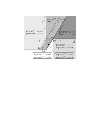
Figure 2: Diagram of the asymptotic behavior of the PDF defined by Eq. (12), in $(s,r)$-plane. Unshadowed regions and dotted borders are regions excluded by the normalization requirement. At both positive semi-axes, the growth at the origin is power law. On dark gray lines, tails are power law, with the tilted line corresponding to $r=2s-1$ ($p=-1$). Dashed lines correspond to pure exponential tails, with the tilted line corresponding to $r=2s$ ($p=0$). In the formulas, $a>0$, as well as the power-law exponents, generically depend on model parameters, moreover $p\equiv r-2s$. Symbols correspond to the special processes A [Eq. (16)] and B [Eq. (18)].

In general, the class of asymptotic behavior is ruled by $(s,r)$ that determine the form of market laws. This holds, of course, as soon as the remaining parameters assume moderate values. For instance, the factor $\lambda^{2}\equiv\gamma_{\alpha}/\gamma_{\mu}$ accompanies $x^{2s}$ in the formula for $\rho(x)$ [Eqs. (12)-(14)], then, extreme values of $\lambda$ will change the asymptotic regime. In fact, in the limit $\alpha=0$ (negligible additive noise, corresponding to $\lambda\to\infty$), different laws arise, as we have seen in the precedent Section.

Summarizing, we have shown the whole picture of asymptotic behaviors that a general class of additive-multiplicative processes produce. As a consequence of the extra additive noise, new types of asymptotic behaviors emerge. Specially interesting solutions arise in the marginal cases $r=0,-1$ where two-fold power-law PDFs are found.

Moreover, additive-multiplicative processes lead to higher richness of crossover behaviors, with respect to purely multiplicative processes. Therefore, the appearance of new PDF shapes exceeds the one resulting from the mere analysis of the asymptotic regimes. This is specially important because depending on the values of the parameters, the true asymptotic regime might fall outside the observable range.

V Comparison with empirical distributions

Let us consider, as paradigm of the PDFs with two-fold power-law behavior, Eqs. (16) and (18), that have a simple exact expression. Actually they have the same functional form, via redefinition of parameters ($\theta,\gamma_{\alpha},\gamma_{\mu}$). This expression has been recently proposed in the literature as an ansatz for fitting the distribution of high-frequency stock-volumes vol1 , under the form

$$\rho(x)=\rho_{o}\frac{(x/x_{o})^{\nu}}{[1+(q-1)x/x_{o}]^{\frac{1}{q-1}}}\;,$$ (19)

where, in that specific application, $x$ is identified with normalized stock volume. Therefore, identification of the process for real volumes with one of the models above, may allow an econophysical interpretation of the fitting parameters. Table I presents the correspondence between the parameters of Eq. (19) and those of processes A and B, given by Eqs. (16) and (18), respectively.

	A	B
Eq. (19)	Eq. (16)	Eq. (18)
$1/(q-1)$	$1+\gamma_{\alpha}\theta+\gamma_{\mu}$	$1+\gamma_{\alpha}+\gamma_{\mu}\theta$
$\nu$	$\gamma_{\alpha}\theta$	$1+\gamma_{\mu}\theta$
$x_{o}$	$(q-1)\gamma_{\mu}/\gamma_{\alpha}$	$(q-1)\gamma_{\alpha}/\gamma_{\mu}$

Table 1: Correspondence amongst model parameters.

Recall that $\gamma_{\alpha}\equiv\gamma/\alpha^{2}$ and $\gamma_{\mu}\equiv\gamma/\mu^{2}$ ($\lambda^{2}\equiv\gamma_{\alpha}/\gamma_{\mu}$), thus, the power-law exponent for small values of $x$, given by $\nu$ (see Table), increases with $\gamma$ and $\theta$, and is reduced by either one of the two noise amplitudes: the additive noise in process A and the multiplicative one in process B. The power-law decay (with exponent $1/(q-1)-\nu$) for large values of $x$ is ruled by either one of the effective coefficients $\gamma_{\mu}$ (in A) or $\gamma_{\alpha}$ (in B) (see Table). That is, the tail is fatter, the larger the corresponding noise amplitude. While in process A the multiplicative noise affects the tail, in model B it is affected by the additive noise, oppositely to what happens for small values. This is related to the sign of $s$, indicating higher multiplicative feedback for either increasing (A) or decreasing (B) values of $x$.

Besides the good agreement already observed for volumes vol1 ; vol2 , we tested this functional form to daily data of volatilities reported in the literaturemicciche . The results are shown in Fig. 3. In the models we are generalizing, the variable $x$ is usually identified with the variance or squared volatility ($x=v^{2}$). Then, the resulting PDF for $v$ is

$$P(v)\;=\;\rho_{o}\frac{(v/v_{o})^{2\nu+1}}{[1+(q-1)(v/v_{o})^{2}]^{\frac{1}{q-1}}}\;,$$ (20)

with $\rho_{o}={\scriptstyle 2(2-q)^{\nu}(q-1)\Gamma(\frac{1}{q-1}-1)/[v_{o}\Gamma(\nu+1)\Gamma(\frac{1}{q-1}-\nu-1)]}$.

Fig. 3 shows an excellent agreement between theoretical and empirical PDFs, for the full range of data. Notice that the very central part of the distribution is parabolic in the log-log plot, then a poor statistics at the tails may mislead to think that the distribution is log-normal.

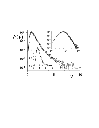
Figure 3: PDF of normalized volatility of stocks traded in US equity market (data from Ref. micciche ). The full line corresponds to a fitting by the theoretical PDF given by expression (20). Fitting parameters are ($q,\nu,v^{2}_{o})\simeq(1.178,2.20,0.097)$. Insets: linear-linear and log-log representation of the same data.

Underlying dynamics

The satisfactory agreement between the empirical data and Eq. (20) suggests that processes similar to either A or B may rule squared-volatility evolution. Hence, let us look at the explicit form of the ILEs associated to processes A and B:

$$\mbox{\bf A:}\;\;\;\;{\rm d}x=-\gamma[x-\theta]\frac{1}{x}{\rm d}t+\mu\sqrt{x}{\rm d}z+\alpha{\rm d}w\,.$$ (21)

$$\mbox{\bf B:}\;\;\;{\rm d}x=-\gamma[x-\theta]\frac{1}{x^{2}}{\rm d}t+\mu\frac{1}{\sqrt{x}}{\rm d}z+\alpha{\rm d}w\,.$$ (22)

The first term in each ILE represents the deterministic restoring force with respect to the level $\theta$. It derives from a confining potential of the form $\gamma[x-\theta\ln x]$ (A) or $\gamma[\ln x+\theta/x]$ (B). In both cases, the potential has a minimum located at $x=\theta$ and is divergent at $x=0$.

Average values are

$$\langle x\rangle_{\bf A}=\frac{\theta+1/\gamma_{\alpha}}{1-1/\gamma_{\mu}}\;\;\;\mbox{and}\;\;\;\langle x\rangle_{\bf B}=\frac{\theta+2/\gamma_{\mu}}{1-2/\gamma_{\alpha}}\;,$$ (23)

both averages are greater than $\theta$ and coincide only in the limit of relatively small noise amplitudes ($\gamma>>\alpha^{2},\mu^{2}$). Moments $\langle x^{n}\rangle$ are finite only if $\gamma_{\mu}>n$ (A) or $\gamma_{\alpha}>n+1$ (B). In particular, the second moment is

$$\langle x^{2}\rangle_{\bf A}=\frac{\gamma_{\alpha}(\theta+1/\gamma_{\alpha})(\theta+2/\gamma_{\alpha})}{\gamma_{\mu}(1-1/\gamma_{\mu})(1-2/\gamma_{\mu})}\;,$$ (24)

$$\langle x^{2}\rangle_{\bf B}=\frac{\gamma_{\mu}(\theta+2/\gamma_{\mu})(\theta+3/\gamma_{\mu})}{\gamma_{\alpha}(1-2/\gamma_{\alpha})(1-3/\gamma_{\alpha})}\;.$$ (25)

In model A, increasing(decreasing) amplitude of the additive(multiplicative) noise, increases the width of the distribution, whereas model B presents opposite behavior. Thus, for instance, the additive noise has a confining effect in process A, opposite to the effect observed in processes with null $\theta$multi1 .

On the other hand, the distribution has a maximum at

$$x^{max}_{\bf A}=\frac{\theta}{1+1/\gamma_{\mu}}\;\;\;\mbox{and}\;\;\;x^{max}_{\bf B}=\theta+\frac{1}{\gamma_{\mu}}\;.$$ (26)

Notice that the additive noise does not affect the mode, as expected. The most probable value of distribution A shifts to the right with increasing multiplicative amplitude, while in distribution B the opposite tendency occurs. From Eqs. (23) and (26), $x^{max}_{\bf A}<\theta_{\bf A}<\langle x\rangle_{\bf A}$, while $\theta_{\bf B}<x^{max}_{\bf B}<\langle x\rangle_{\bf B}$. That is, in model A, the reference value $\theta$ represents a typical value comprised between two central measures, which does not hold in model B. This observation, in addition to the positivity of $s$, point to model A as a more realistic long-term process.

The fitting parameters in Fig. 3 lead to ($\theta,\gamma_{\mu},\gamma_{\alpha})_{\rm\bf A}\simeq(0.50,2.4,4.4)$ or ($\theta,\gamma_{\mu},\gamma_{\alpha})_{\rm\bf B}\simeq(0.19,6.3,3.4)$. In both cases, $\gamma_{\mu},\gamma_{\alpha}>1$, as expected for regulated markets. While $\langle v\rangle=1$, because empirical volatility is normalized, $\langle x\rangle=\langle v^{2}\rangle\simeq 1.3$ and the mode is $x^{max}\simeq 0.35$, consistently with Eqs. (23)-(26).

Numerical integration of ILEs (21) and (22), by standard methodsbooks , shows that both processes produce time series with bursting or clustering effects, as observed in real sequences. However, process B may present, for some values of the parameters, a kind of ergodicity breaking, with large jumps to a state basically governed by additive noise. This occurs because, once $x$ jumps to a high value, both the restoring force and the effective amplitude of multiplicative noise become small as to pull $x$ back to its reference level. Then, relaxation is slowed down and the regime of high volatility persists for long time stretches. Although a process with $s<0$ is not expected to be a realistic model for very long time intervals, it can model, for instance, the transient behavior of the market around crashes. In fact, process B yields akin crises. After the crash occurs, this drastic event might switch the system back to a $s\geq 0$ regime.

VI Final remarks

We have analyzed stochastic models of a quite general form, with algebraic restoring force and algebraic multiplicative noise. A further generalization with the inclusion of an extra source of noise, of standard Wiener type, has also been analyzed. These additive-multiplicative processes are built on the basis of realistic features: The multiplicative noise describes innovations generated by endogenous mechanisms that amplify or attenuate a random signal, depending on the internal state of the system. Whereas, the additive noise encodes a direct influence of external random fields such as news or spontaneous fluctuations due to speculative trading. One of the goals of this work was to study systematically the PDF asymptotic solutions of these generalized models. We have shown that the inclusion of additive noise gives rise to new PDF shapes, with a richer spectrum of cross-over behaviors and, in particular, two-fold power-law decays. The shapes of the PDFs are governed by the effective market rules parametrized by $r$ and $s$. These parameters describe the algebraic nature of the global mean-reverting strength of the market and the informational coupling among the traders, respectively. On the other hand, power-law exponents and coefficients of exponential-like functions depend also on the reduced parameters $\gamma_{\mu}$, $\gamma_{\alpha}$ and on $\theta$. This means that one may expect universal behavior among markets that share similar rules (same $r$ and $s$) and same rescaled restoring parameters, for a properly normalized reference level $\theta$. Summarizing, the additive-multiplicative processes given by Eq. (10) provide a general realistic framework to describe the shape of empirical distributions for financial, as well as, for physical systems. An illustrative application to empirical volatility data was presented in Sect. V, showing excellent results.

The statistical description of a market should include its dynamical properties such as the temporal decay of correlations. In real time series of volatilitiesliu and volumesvolumes , power-law decaying correlations have been observed. It is worth noting that stochastic processes with additive-multiplicative structure (without mean reversion) are being currently studied in connection with a generalization of standard (Boltzmann-Gibbs) statistical mechanics, recently proposed by C. Tsallis tsallis . The PDFs associated to this new formalism generalize the exponential weights, namely, $\exp_{q}(-x)\equiv(1-[1-q]x)^{\frac{1}{1-q}}$ [entering as a factor in Eq. (19)]. The time series arising from additive-multiplicative processes without mean reversion present strong correlations that prevent convergence to either Gauss or Lévy limitsmulti3 and lead to $q$-Gaussian distributions. This suggests that similar correlations may persist in mean-reverting processes with the additive-multiplicative character. Once Eq. (10) leads to PDFs in such a good agreement with empirical ones, it is worth performing a detailed study and comparison of real and artificial time series to test the models with respect to the dynamics. Elucidating this point deserves a careful separate treatment.

Acknowledgments: We are grateful to S. Miccichè, G. Bonanno, F. Lillo and R.N. Mantegna for communicating their numerical data in Ref. micciche .

References

- (1) J.P. Fouque, G. Papanicolaou and K.R. Sircar, Derivatives in financial markets with stochastic volatility (Cambridge U.P., Cambridge, 2000).
- (2) P. Gopikrishnan, V. Plerou, L.A.N. Amaral, M. Meyer and H.E. Stanley, Phys. Rev. E 60, 5305 (1999); L. Borland, Phys. Rev. Lett. 89, 098701 (2002); M. Ausloos and K. Ivanova, Phys. Rev. E 68, 046122 (2003); L. Borland, J.-P. Bouchaud, J.-F. Muzy and G. Zumbach, cond-mat/0501292.
- (3) J.-P. Bouchaud, A. Matacz and M. Potters, Phys. Rev. Lett. 87, 228701 (2001).
- (4) Y. Liu, P. Gopikrishnan, P. Cizeau, M. Meyer, C.K. Peng, H.E. Stanley, Phys. Rev. E 60, 1390 (1999).
- (5) T. G. Andersen, T. Bollersev, F. X. Diebold, H. Ebens, J. Financial Econom. 63, 43 (2001).
- (6) S. Miccichè, G. Bonanno, F. Lillo and R. Mantegna, Physica A 314, 756 (2004).
- (7) P. Gopikrishnan, V. Plerou, X. Gabaix, H.E.Stanley, Phys. Rev. E 62, R4493 (2000).
- (8) R. Osorio, L. Borland and C. Tsallis, in: M.Gell-Mann,C.Tsallis (Eds.), Nonextensive Entropy Interdisciplinary Applications, (Oxford University Press, Oxford, 2003).
- (9) C. Tsallis, C. Anteneodo, L. Borland and R. Osorio, Physica A 324, 89 (2003).
- (10) J. Hull and A. White, Rev. Financial Studies 3, 573 (1990); J.C. Cox, J.E. Ingersoll and S.A. Ross, Econometrica 53, 385 (1985).
- (11) J. Hull and A. White, J. Finance 42, 281 (1987).
- (12) S.L. Heston, Review of Financial Studies 6, 327 (1993).
- (13) J.C. Cox, J.E. Ingersoll and S.A. Ross, Econometrica 53, 363 (1985).
- (14) W. Feller, Annals of Mathematics 54, 173 (1951).
- (15) J.P. Fouque, G. Papanicolaou and K.R. Sircar, Int. J. Theor. Appl. Finance 3, 101 (2000); A.A. Drăgulescu and V.M. Yakovenko, Q. Finance 2, 443 (2002); E.M. Stein and J.C. Stein, Review of Financial Studies 4, 727 (1991); D.S. Bates, Review of Financial Studies 9, 69 (1996);
- (16) H. Risken, The Fokker-Planck Equation. Methods of Solution and Applications (Springer-Verlag, New York, 1984); C. W. Gardiner, Handbook of Stochastic Methods, (Springer, Berlin, 1994).
- (17) A. Schenzle and H. Brandt, Phys. Rev. A 20, 1628 (1979).
- (18) C. Anteneodo and C. Tsallis, J. Math. Phys. 44, 5203 (2003).
- (19) H. Sakaguchi, J. Phys. Soc. Jpn. 70, 3247 (2001).
- (20) C. Anteneodo, preprint cond-mat/0409035 (2004).
- (21) D. Sornette, Y. Malevergne and J.-F. Muzy, cond-mat/0204626.
- (22) A. Krawiecki, J.A. Holyst and D. Helbing, Phys. Rev. Lett. 89, 158701 (2002).
- (23) M. Abramowitz and I. A. Stegun, Handbook of Mathemat- ical Functions with Formulas, Graphs, and Mathematical Tables, National Bureau of Standards, Applied Mathemat- ics Series 55 (Washington, 1965).
- (24) The hypergeometric function behaves asymptotically as , for small , and as ), if , for large .
- (25) C. Tsallis, J. Stat. Phys. 52, 479 (1988). Nonextensive Statistical Mechanics and its Applications, edited by S. Abe and Y. Okamoto, Lecture Notes in Physics Vol. 560 (Springer-Verlag, Heidelberg, 2001); Anomalous Distributions, Nonlinear Dynamics and Nonextensivity, edited by H. L. Swinney and C. Tsallis [Physica D (2004)]. Nonextensive Entropy - Interdisciplinary Applications, edited by M. Gell-Mann and C. Tsallis (Oxford University Press, New York, 2004).