FIELD OF THE CURRENT PULSE MOVING
ALONG THE STRAIGHT LINE WITH SUPER LIGHT VELOCITY.

Abstract   A simulation of electric current pulses formed by a packet of gamma-quanta moving through an absorptive medium is presented. The electromagnetic fields of the current pulse moving along the straight line with super light velocity are obtained.

1 Introduction

In recent years the electromagnetic fields of sources moving with velocities equal or higher than velocity of light c in vacuum have been discussed in connection with an interest to the problem of localized electromagnetic waves [1, 2]. Such a source can be obtained by interaction of a directed beam of a hard electromagnetic radiation (X-rays) with an absorptive rod. It is important to have the length of this rod larger than its diameter. If initial quanta are moving along the axis of this rod, the electron’s current pulse whose velocity is equal to c is generated. If the beam is directed at an angle to the rod’s axis, the current pulse has a super light velocity. The velocities of electrons, of course, are smaller than c, but the motion of area, where the current’s density is non zero, can be presented as the motion of some effective charge which is faster than the velocity of light in vacuum. The investigation of the spatial structure and of the time dependence of secondary electromagnetic fields, generated by such a pulse, requires solution of two problems. Firstly, we have to find the shape of the current pulse generated by the beam of primary hard electromagnetic radiation. Secondly, we have to solve the Maxwell’s equation for this current’s pulse with zero initial conditions. The current pulse in question was earlier studied mainly on a phenomenological basis. The current pulse moving with velocity of light was considered in connection with nuclear explosions [3].
In this paper we calculate the “realistic” shape of current pulse moving with super-light velocity, taking into account the microscopic movements of the electrons. We obtained electromagnetic fields with this current pulse by using the approach presented in [4], based on the method of an incomplete separation of variables by V.I. Smirnov [5] and Riemann formula.

2 The shape of the super-luminal current
pulse generated by a shot-lived beam of a hard radiation

The solution of the first problem of finding the shape of current pulse requires to take into account the photon absorption’s processes, Compton scattering, and secondary coupling effects of “delta electrons” with matter which result in the formation of the ions and the electrons. We found the shape of current pulse via the computational experiment using the method of numerical modelling described in [6]. This method enables us to study the time dependence of the electrons’ distribution in the phase space. The code GEANT [7] was used. The generation of the electrons with energy lower than 10 keV was not taken into account.

The scheme and the initial conditions of the computational experiment are as follows. The absorbing area is placed in vacuum and is bounded by the cylindrical surface of 0.3 m. in diameter and of 50 m. in length L and by the two planes, which are orthogonal to the cylinder axis. Its walls are made of hydrocarbon-based material. Their thickness is 0.001 m. The absorptive medium is air at the pressure of 1 atm. The symmetry axis of the absorbing area coincides with the axis z of a cylindrical coordinate system .

The origin of the coordinate system is chosen to be localized at the point O, which lies in one of the two above mentioned planes.

The packet of the primary photons (a gamma-ray pulse) starts from a surface formed by rotation of a line segment, which is at an angle $\pi$/2- $\theta$ to the Z axis . The photons are simultaneously emitted at an angle $\theta$ to the direction of the z axis.

The computational experiment is beginning with the starting time of the gamma-ray pulse. The results of computer experiments are as follows:

1. We obtained the distribution N($\rho)$ of the secondary photoelectrons which have passed through the plane fixed at z=z₀. This distribution describes the electron localization in the radial direction $\rho$.

2. The width ($\Delta$R) of the distribution N($\rho)$ calculated for the above initial conditions is less than 30 centimeters ($\Delta R<30cm$). The obtained value meets the necessary requirement of the applicability of the model of a linear current ($L>>\Delta R$), used in the simplified electrodynamic calculations.

The time dependence of the current’s pulse passing through the absorptive area at $z_{0}=30$ meters is shown in Fig. 1.

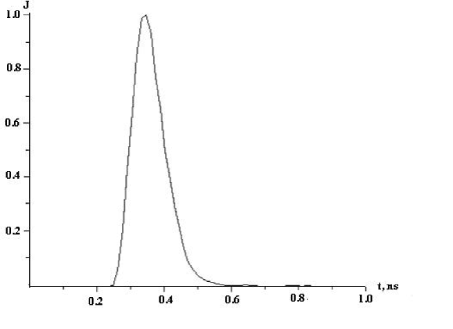
Figure 1: The normalized current pulse in the cross section of the absorbing region at z = 30 m.

In this plot the value of function in maximum is presented as 1.0 on the axis of ordinates. The pulse length ($\Delta$T) taken on the ordinates level of 0.1 does not exceed 0.2 ns (or 6 cm in ct - units). The obtained value of $\Delta$T estimates the localization of the current along z – axis.

The shape of the running pulse can be described by the following function:

$$J(z,\tau)=A\cdot(1-\exp(-\alpha_{1}(\beta\tau-z)))\cdot\exp(-\alpha_{2}(\beta\tau-z))$$ (1)

$\alpha_{i}>0$, i=1,2,

where $\tau=ct$ is the time variable, $\beta=v/c$ , $A$ is constant ; coefficients $\alpha_{i}$ are obtained by the least square method

Thus, as a result of the above computational experiment the space-time description of the hard radiation inducing super light running pulse was obtained.

3 Calculation of the magnetic component of the electromagnetic wave generated by the current pulse moving with super light velocity

The basic solution of the Maxwell equations that describes waves generated by a current pulse propagating along the section of a strait line was given in [2]. In that work the components of both the electric and magnetic fields are expressed via a single scalar function $v(\rho,z,\tau)$. In the present work we represent only magnetic component B. That was made to simplify the subsequent physical interpretation of the obtained results.

In our case the parameters of the hard radiation and absorptive medium, geometry of the absorptive area were chosen in accordance with the condition $L>>\Delta R$. The boundary effects in the description of a source of electrodynamics problem are not taken into account (the necessary requirement $L>>\Delta T$ is met). This means that for the calculation of the required electromagnetic field (its magnetic component) we may use the simplified model of a linear current.

Thus the source in the electrodynamics problem (non-zero component of the current’s density vector) can be taken in the form:

$$j_{z}={\frac{{\delta(\rho)}}{{2\pi\rho}}}h(\beta\tau-z)h(z)h(L-z)J(z,\tau)\quad\tau>0\quad_{,}$$ (2)

$$j_{z}=0\quad\tau<0$$

Here $\delta(\rho)$ is the Dirac distribution, h(z) is the Heaviside step function.  In the case of the axial - symmetric source of an electrodynamics problem, the components of the intensity E of electric field and the induction B of magnetic field may be expressed via one scalar function $v$ according to the following expressions:

$$E_{\rho}={\frac{{\partial^{2}u}}{{\partial\rho\partial z}}}\quad E_{z}=-{\frac{{\partial^{2}u}}{{\partial\tau^{2}}}}+{\frac{{\partial^{2}u}}{{\partial z^{2}}}}\quad B_{\varphi}={\frac{{\partial^{2}u}}{{\partial\tau\partial\rho}}}\quad_{,}$$ (3)

Now the electrodynamics problem can be expressed in the form:

$$\left({\frac{\partial^{2}}{\partial\tau^{2}}-\frac{1}{\rho}\frac{\partial}{\partial\rho}\left({\rho\frac{\partial}{\partial\rho}}\right)-\frac{\partial^{2}}{\partial z^{2}}}\right)v=\frac{4\pi}{c}j_{z},j_{z}=0\tau<0_{,}$$ (4)

were $v=\partial u/\partial\tau$  The non-zero component of the magnetic induction $B_{\varphi}$vector is equal to$-\partial v/\partial\rho$.

The solution of the problem (4) in space - time representation is defined by the following expression:

$$v(\rho,z,\tau)={\frac{1}{c}}\int\limits_{0}^{\tau}{d\tau}\int\limits_{\tau^{\prime}+z-\tau}^{-\tau^{\prime}+z+\tau}{dz^{\prime}h(z^{\prime})}$$ (5)

$$h(\beta\tau^{\prime}-z^{\prime})h(L-z^{\prime})J(z^{\prime},\tau^{\prime}){\frac{{\delta(\tau^{\prime}-\tau+\sqrt{\rho^{2}+(z-z^{\prime})^{2}})}}{\sqrt{\rho^{2}+(z-z^{\prime})^{2}}}}$$

After interchanged the order of an integration, we receive:

$$v(\rho,z,\tau)={\frac{1}{c}}\int\limits_{z-\tau}^{z}{dz^{\prime}}h(z^{\prime})h(L-z^{\prime}){\frac{1}{\sqrt{\rho^{2}+(z-z^{\prime})^{2}}}}I_{1}$$

$$\quad+{\frac{1}{c}}\int\limits_{z}^{z+\tau}{dz^{\prime}}h(z^{\prime})h(L-z^{\prime}){\frac{1}{\sqrt{\rho^{2}+(z-z^{\prime})^{2}}}}I_{2}$$ (6)

where

$$I_{1}=\int\limits_{0}^{-z^{\prime}+\tau-z}{d\tau^{\prime}J(z^{\prime},\tau^{\prime})h(\beta\tau^{\prime}-z^{\prime})\delta(\tau^{\prime}-\tau+\sqrt{\rho^{2}+(z-z^{\prime})^{2}})}$$

$$I_{2}=\int\limits_{0}^{-z^{\prime}+\tau+z}{d\tau^{\prime}J(z^{\prime},\tau^{\prime})h(\beta\tau^{\prime}-z^{\prime})\delta(\tau^{\prime}-\tau+\sqrt{\rho^{2}+(z-z^{\prime})^{2}})}$$

For a super light delta - pulse

$$j_{z}={\frac{{\delta(\rho)}}{{2\pi\rho}}}\delta(\beta\tau-z)h(z)h(l-z)f(z,\tau)$$

(where $f$ is differentiable function) expression (6) can be simplified

$$v(\rho,z,\tau)={\frac{1}{c}}(\psi_{1}+\psi_{2})$$

Here

$$\psi_{1}(\rho,z,\tau)=$$

$$f\left(\beta\left(\frac{\beta z-\tau+\sqrt{D}}{\beta^{2}-1}\right),\frac{\beta z-\tau+\sqrt{D}}{\beta^{2}-1}\right)\frac{1-h(\sqrt{D}+(1-\beta^{2})\tau-\beta(z-\beta\tau))}{\sqrt{D}}$$

$$\times\{[h(L)(h(z-\tau)-h(z+\tau))]$$

$$\times[h(\beta(\sqrt{D}-z\beta+\tau))-h(-z\beta^{2}+L(-1+\beta^{2})+\beta(\sqrt{D}+\tau))]$$

$$+h(L-z-\tau)h(z+\tau)$$ (7)

$$\times[h(-z+\sqrt{D}\beta+(-1+\beta+\beta^{2})\tau)-h(-z{\beta^{2}+L(-1+\beta^{2})+\beta(\sqrt{D}+\tau)})]$$

$$+h(z-\tau)h(L-z+\tau)$$

$$\times[-h(-z+\sqrt{D}\beta+(1+\beta-{\beta^{2}})\tau)+h(-z\beta^{2}+L(-1+\beta^{2})+\beta(\sqrt{D}+\tau))]\}$$

,

$$\psi_{2}(\rho,z,\tau)=$$

$$\times f\left(\beta\left(\frac{\beta z-\tau-\sqrt{D}}{\beta^{2}-1}\right),\frac{\beta z-\tau-\sqrt{D}}{\beta^{2}-1}\right)\frac{1-h(\sqrt{D}+(1-\beta^{2})\tau+\beta(z-\beta{\tau}))}{\sqrt{D}}$$

$$\times\{[h(L)(h(z-\tau)-h(z+\tau))]$$

$$\times[h(-\beta(\sqrt{D}+z\beta-\tau))-h(-z\beta^{2}+L(-1+\beta^{2})+(\beta-\sqrt{D}+\tau))]$$ (8)

$$+h(L-z-\tau)h(z+\tau)$$

$$\times[h(-z+\sqrt{D}\beta-(-1+\beta+\beta^{2}))\tau-h(-z\beta^{2}+L(-1+\beta^{2})+\beta(-\sqrt{D}+\tau))]$$

$$+h(z-\tau)h(L-z+\tau)$$

$$\times[-h(-z+\sqrt{D}\beta+(-1-\beta+\beta^{2})\tau)+h(-z{\beta^{2}+L(-1+\beta^{2})+\beta(-\sqrt{D}+\tau)})]\},$$

where $D=(z-\beta\tau)^{2}-\rho^{2}(\beta^{2}-1)$. This expression may be used also for the nondispersive matter ($\beta$ is the ratio of velocity of the source motion to the light velocity in given environment in this case).

We carried out the numerical calculation of super light source using the expression (6). The time dependence of $v(\rho,z,\tau)$ is presented on fig. 2 for the seven angles of gamma - quanta.

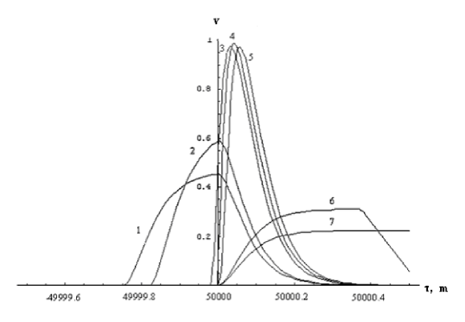
Figure 2: Time dependence (in $ct$ units) of $v(\rho,z,\tau)$ normalized to the maximal amplitude of different observation angles $\theta=0.3^{0}$(1), $\theta=3^{0}$(2), $\theta=5.5^{0}$,$\theta=5.44^{0}$(1), $\theta=\arccos(c/v)=arctg(0.1)\approx 5.71^{0}$(4), $\theta=6^{0}$(5),$\theta=9^{0}$(6),$\quad\theta=10^{0}$(7)

In the proximity of the angle $\theta=\arccos(c/v)=5.71^{0}$ the function $v(\rho,z,\tau)$sharpens its form. Note, that the variation of parameters of numerical experiment causes essential changes of $v(\rho,z,\tau)$ . In particular, the reduction of value of $L$ results in disappearance of a characteristic maximum in the distribution $v(\theta)$ at $\theta=\arccos(c/v)$. The dependence of $B_{\varphi}$ component on $\tau$ at various angles of observation $\theta$ ($L=50m$, $Z=50000m$) is presented in Fig.3.

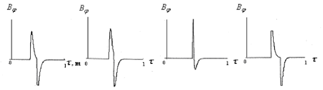
Figure 3: $B_{\varphi}$ components of magnetic induction at various angles of observation $\theta=0.3^{0}$(1), $\theta=3^{0}$(2) , $\theta=\arccos(c/v)=arctg(0.1)\approx 5.71^{0}$, $\theta=6^{0}$(4),$\theta=9^{0}$(5)$\quad\theta=10^{0}$(6) and $L=50m$, $Z=50000m$

As we see, duration of the two-polar pulses of an electromagnetic field depends on angle $\theta$. The reduction of duration and the growth of amplitude of the first half-wave in the vicinity of $\theta=\arccos(c/v)$ is observed. The representation $B_{\varphi}(\rho,z,\varphi,\tau)$ by Fourier integral allowed us to obtain the frequency distribution of energy of the electromagnetic field for different values of observation angles in a far zone. The frequency spectra of electromagnetic pulses for observation angles : $\theta=0.3^{0}$, $\theta=3^{0}$ , $\theta=5.5^{0}$ ,$\theta=5.44^{0}$, $\theta=\arccos(c/v)=arctg(0.1)\approx 5.71^{0}$, $\theta=6^{0}$,$\theta=9^{0}\quad\theta=10^{0}$ in the optical range are presented in Fig. 4.

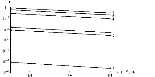
Figure 4: The energy spectra of electromagnetic pulse observed at various angles $\theta=6.4^{0}$(1), $\theta=0.3^{0}$(2), $\theta=3^{0}$ , $\theta=5.5^{0}$ (4) , $\theta=5.8^{0}$(5), $\theta=\arccos(c/v)=arctg(0.1)\approx 5.71^{0}$(6) in the far zone ( $Z=50000m)$ in optical frequency range ($3\ast 10^{14}-8\ast 10^{14})$ Hz for $v/c\cong 1.005$.

As we see, radiation at the angle $\theta=\arccos(c/v)$ to the direction of current pulse motion in the visible range of a spectrum has maximal value.

4 Summary

We have calculated the shape of a the current pulse moving with velocity greater then the velocity of light in vacuum for the certain geometry of the hard radiation at fixed values of parameters of gamma - quanta pulse moving through a layer of air.

The analytic representation for the potential $v(\rho,z,\tau)$ was obtained for the case of the superluminal delta pulse.

The spectra of radiation in the optical range for some different observation angles range for $v/c$ equal 1.005 were calculated. We found that the radiation has maximum at $\theta\cong\arccos(c/v)$.

References

- [1] E. Recami . Foundations of Physica 31.No.7 1119(2001).
- [2] Borisov V.V., Utkin A.B. J.Phys.D.: Appl.Phys 614(1995)
- [3] Karzas W.J., Letter R Phys.Rev. B., , 137(5) , 1369(1965).
- [4] Manankova A.V. Izv.Vyssh.Uchebn.Zaved.Radiofiz,15, 211(1972).
- [5] V.I. Smirnov A Course of Higher Mathematics, Vol.4. (Nauka press,Moskow,1965).
- [6] F.F.Valiev Tech. Phys.,46. No.12 1579(2001).
- [7] User’s Guide. CERN DD/EE/83-1 (1983)