Topology hidden behind the breakdown of adiabaticity

Abstract

For classical Hamiltonian systems, the adiabatic condition may fail at some critical points. However, the breakdown of the adiabatic condition does not always make the adiabatic evolution be destroyed. In this paper, we suggest a supplemental condition of the adiabatic evolution for the fixed points of classical Hamiltonian systems when the adiabatic condition breaks down at the critical points. As an example, we investigate the adiabatic evolution of the fixed points of a classical Hamiltonian system which has a number of applications.

I Introduction

Adiabaticity is an interesting concept in physics both for theoretical studies and experimental practices book ; book1 ; book3 ; adiab ; adiab1 . According to the adiabatic theorem book , if the parameters of the system vary with time much more slowly than the intrinsic motion of the system, the system will undergo the adiabatic evolution. For a classical system, the adiabatic evolution means that the action of the trajectory keeps invariant. For a quantum system, an initial nondegenerate eigenstate remains to be an instantaneous eigenstate when the Hamiltonian changes slowly compared to the level spacings book . Hence, the adiabatic evolution has been employed as an important method of preparation and control of quantum states adiaba ; bergmann ; raizen ; comp .

However, a problem may arise when the eigenstates become accident degenerate at a critical point, i.e., when the level spacing tends to zero at a critical point. For a classical system it corresponds to that the frequency of the fixed point is zero at the critical point. The adiabatic condition is not satisfied at the critical point because the typical time of the intrinsic motion of the system becomes infinite. Can adiabatic evolution still hold up when the adiabatic condition breaks down at the critical point?

Our motivation, derives from practical applications in current pursuits of adiabatic control of Bose Einstein condensates (BECs) bec , which can often be accurately described by the nonlinear Schrödinger equation. Here the nonlinearity is from a mean field treatment of the interactions between atoms. Difficulties arise not only from the lack of unitarity in the evolution of the states but also from the absence of the superposition principle. This was recently addressed for BECs in some specific cases band ; kivshar . But then, however, for such systems, only finite number of levels are concerned. The nonlinear Schrödinger equation of the system with finite number of levels can be translated into a mathematically equivalent classical Hamiltonian system. The evolution of an eigenstate just corresponds to the evolution of a fixed point of the classical Hamiltonian system. Then, the accident degeneracy of eigenstates is just translated into accident collision of the fixed points. The latter one is quite well-known subject and has been studied widely at least as a purely mathematical problem book2 . Hence, our concern here is only focused on the adiabatic evolution of the fixed points of classical Hamiltonian systems.

In this paper, we present a supplemental condition of the adiabatic evolution for the fixed points of classical Hamiltonian systems when the adiabatic condition breaks down at some critical points in the terms of topology. As an example, we investigate the adiabatic evolution of the fixed points of a classical Hamiltonian system which has a number of practical interests. We show that the adiabatic condition will break down at bifurcation points of the fixed points. But the adiabatic evolution is destroyed only for the limit point. For the branch process, the adiabatic evolution will hold, and the corrections to the adiabatic approximation tend to zero with a power law of the sweeping rate.

II Supplemental adiabatic condition for the fixed points of classical Hamiltonian systems

For clarity and simplicity, we consider a one-freedom classical Hamiltonian $H(p,q;\lambda)$ with canonically conjugate coordinates $(p,q)\;$where $\lambda$ is a parameter of this system. The equations of motion are:

$$\overset{.}{q}=\frac{\partial H}{\partial p},\;\overset{.}{p}=-\frac{\partial H}{\partial q}.$$ (1)

We can find two kinds of trajectories in the phase space for the system: fixed points and closed orbits. The fixed points are the solutions of Eqs. (1) when the right hands of them are zero. For a Hamiltonian system there are only two kinds of the fixed points: elliptic points (stable fixed points), hyperbolic points (unstable fixed points). The closed orbits are around each of the elliptic points. We denote the fixed points by $z_{i}^{\ast}(p,q)\;(i=1,2,\cdots,l)$ where $l$ is the total number of the fixed points.

The action of a trajectory is defined as

$$I=\frac{1}{2\pi}\oint pdq,$$ (2)

where the integral is along the closed orbit. Obviously, the action of a fixed point is zero. The action is invariant when system undergos adiabatic evolution.

According to the adiabatic theorem book , the adiabatic condition can be expressed as

$$\frac{2\pi}{\Omega}\frac{d\lambda}{dt}<<1,$$ (3)

where $\Omega$ is the frequency of the fixed point. If this condition holds, the system will undergo adiabatic evolution, and keep the action not varying. If $\Omega\neq 0,$ the condition can always be satisfied.

We can obtain the frequencies of the fixed points by linearized the equations of motion. Let us define the Jacobian matrix as

$$J=\left(\begin{array}[]{cc}\frac{\partial^{2}H}{\partial q^{2}}&\frac{\partial^{2}H}{\partial q\partial p}\\ \frac{\partial^{2}H}{\partial q\partial p}&\frac{\partial^{2}H}{\partial p^{2}}\end{array}\right).$$ (4)

It is well-known that when $\det(J)|_{z^{\ast}}>0,$ the fixed point is a stable fixed point (elliptic point); when $\det(J)|_{z^{\ast}}<0,$ the fixed point $z^{\ast}$ is a unstable fixed point (hyperbolic point). The point with $\det(J)|_{z^{\ast}}=0$ is a degenerate point at which the stability of the system is not determined.

For a stable fixed point $z^{\ast},$ the frequency of this fixed point is

$$\Omega_{0}=\sqrt{|\det(J)|_{z^{\ast}}}.$$ (5)

Obviously, $\Omega_{0}$ depends on the parameter $\lambda.$

Supposing at a critical point, namely $\lambda=\lambda_{c},$ we have $\Omega_{0}(\lambda_{c})=0.$ Therefore, the condition (3) will break down at the point. We want to know what will happen when the adiabatic condition fails (will the adiabatic evolution of the fixed point be destroyed when the adiabatic condition does not hold ?).

In fact, if $|\det(J)|_{z^{\ast}}=0,$ the point $z^{\ast}$ is a bifurcation point at which the fixed point will collide with the other fixed points book2 ; fu . Hence, the breakdown of adiabatic condition is equivalent to collision of the fixed points (equivalent to accident degeneracy of eigenstates of a corresponding quantum system). In the collision process, fixed points may annihilate or merge into a stable fixed point. The collision of the fixed points can be described clearly in the terminology of topology fu .

The equations of motion just define a tangent vector field $\mathbf{\phi}(p,q)=(\frac{\partial H}{\partial p},-\frac{\partial H}{\partial q})$ on the phase space. Obviously, the fixed points $z_{i}^{\ast}(i=1,2,\cdots l)$ are the zero points of the vector field, i.e., $\mathbf{\phi}(z^{\ast})=0$. We know that the sum of the topological indices of the zero points of the tangent vector field is the Euler number of the phase space which is a topological invariant lisheng . For a Hamiltonian system, the topological index for a stable fixed point is $+1$ and for a unstable fixed point is $-1.$

Indeed, if the fixed point is a regular point (not a degenerated point), i.e., $\det(J)|_{z^{\ast}}\neq 0$, the topological index of the fixed point can be determined by determinant of the Jacobian matrix defined by Eq. (4) lisheng ; fu . If $\det(J)|_{z^{\ast}}>0$, $z^{\ast}$ is a stable fixed point and the topological index is $+1$; if $\det(J)|_{z^{\ast}}<0,$ it is a unstable fixed point and the index is $-1.$

If $\det(J)|_{z^{\ast}}=0,$ i.e. if $z^{\ast}$ is a bifurcation point, the topological index of this point seems to be not determined. As we have shown before, the point is just the critical point of adiabatic evolution, corresponding to collision of the fixed points.

However, because the sum of the topological indices is a topological invariant, the topological index is conserved in a collision process of the fixed points. Therefore, the topological index of the bifurcation point can be determined by the sum of the indices of the fixed points involved in collision. So, if the topological index of the bifurcation point is not zero, it is still a fixed point after collision. But if the topological index of the bifurcation point is zero, the bifurcation point will not be a fixed point after collision.

Now, let us imagine what will happen when a fixed point is destroyed by a collision process. Because there are only two kinds of trajectories for a classical Hamiltonian system: fixed points and closed orbits around each of the stable fixed point, so when a fixed point is destroyed, it will form a closed orbit around the nearest stable fixed point. The action of the new orbit must be proportional to the distance between the critical point and the nearest stable fixed point. This sudden change of action (from zero to finite) is so-called ”adiabatic tunneling probability” which has been studied in Refs. wuniu ; add . On the other hand, if the topological index of the bifurcation point is $-1$, i.e., it is a unstable fixed point after the collision, we can not expect the adiabatic evolution can keep on after collision.

But if the topological index of the bifurcation point is $+1$, i.e., it is still a stable fixed point after the collision, or in other word, the stable fixed point survive after collision. For such case, the adiabatic evolution will not be destroyed.

From above discussion, it is clear that when the adiabatic condition given by Eq. (3) does not hold at a critical point with $\Omega_{0}=\sqrt{|\det(J)|_{z^{\ast}(\lambda_{c})}}=0,$ the system will still undergo the adiabatic evolution if the topological index of the fixed point $z_{\ast}(\lambda_{c})$ is $+1$. On the contrary, if the topological index of the point $z_{\ast}(\lambda_{c})$ is zero or $-1$ the adiabatic evolution will be destroyed.

Hence, we get a supplemental condition of the adiabatic evolution of the fixed points for a classical Hamiltonian system when the adiabatic condition breaks down at a critical point. When the adiabatic condition is not satisfied at a critical point, the topological property of the bifurcation point plays an important role to judge whether the system will undergo adiabatic evolution over this critical point: if the index of the degenerated point $z_{\ast}(\lambda_{c})$ is $+1$ the adiabatic evolution will hold. If the index of the point $z_{\ast}(\lambda_{c})$ is zero or $-1$, the adiabatic evolution will not hold.

III A paradigmatic example and application

As a paradigmatic example, we consider the following system

$$H(z,\theta,\lambda,\gamma)=-\sqrt{1-z^{2}}\cos\theta-\frac{\lambda}{2}z^{2}+\gamma z,$$ (6)

in which $(z,\theta)$ are canonically conjugate coordinates, and $\lambda$, $\gamma$ are two parameters. The equations of motion are : $\dot{\theta}=\frac{\partial H}{\partial z},\;\dot{z}=-\frac{\partial H}{\partial\theta}$, these yield

$$\dot{\theta}=\frac{z}{\sqrt{1-z^{2}}}\cos\theta-\lambda z+\gamma,$$ (7)

$$\dot{z}=-\sqrt{1-z^{2}}\sin\theta.$$ (8)

This classical system can be obtained from a quantum nonlinear two-level system, which may arise in a mean-field treatment of a many-body system where the particles predominantly occupy two energy levels. For example, this model arises in the study of the motion of a small polaron liufu6 , a Bose-Einstein condensate in a double-well potential liufu7 ; liufu8 ; liufu9 or in an optical lattice liufu10 ; liufu11 , or for two coupled Bose-Einstein condensates lee ; fupla , or for a small capacitance Josephon junction where the charging energy may be important. This quantum nonlinear two-level model has also been used to investigate the spin tunneling phenomena recently liufub .

The fixed points of the classical Hamiltonian system are given by the following equations

$$\theta^{\ast}=0,\pi,\;\;\;\gamma-\lambda z^{\ast}+\frac{z^{\ast}}{\sqrt{1-z^{\ast 2}}}\cos\theta^{\ast}=0.$$ (9)

The number of the fixed points depends on the nonlinear parameter $\lambda.$ For weak nonlinearity, $\lambda\leq 1,$ there exist only two fixed points, corresponding to the local extreme points of the classical Hamiltonian. They are elliptic points located on lines $\theta^{\ast}=$ $0$ and $\pi$ respectively, each being surrounded by closed orbits. For strong nonlinearity, $\lambda>1,$ two more fixed points appear on the line $\theta^{\ast}=$ $0$ in the windows $-\gamma_{c}<\gamma<\gamma_{c},$ one is elliptic and the other one is hyperbolic as a saddle point of the classical Hamiltonian, where $\gamma_{c}=(\lambda^{2/3}-1)^{3/2}.$ In the following, we only consider the cases in the region $-\gamma_{c}<\gamma<\gamma$.

We can obtain the frequencies of the fixed points by linearized the Eqs. (7) and (8). For the elliptic fixed points on line $\theta^{\ast}=$ $0,$ the frequencies are equal, they are

$$\Omega_{0}=\sqrt{1-\lambda(1-z^{\ast 2})^{3/2}}.$$ (10)

Obviously, if $z^{\ast}=z_{c}^{\ast}=\sqrt{1-\left(\frac{1}{\lambda}\right)^{2/3}},$ the frequencies will be zero, i.e., $\Omega_{0}(z_{c}^{\ast})=0$. From Eq. (9), we can obtain, when $\lambda=\lambda_{c}=$ $(\gamma^{2/3}+1)^{3/2},$ one of the elliptic fixed point will be $(z^{\ast}=z_{c}^{\ast},\theta^{\ast}=0).$ At this point the adiabatic condition will break down.

Hence, if we start from this elliptic fixed point on line $\theta^{\ast}=$ $0$ at $\lambda=\lambda_{0}>1$, and $\lambda$ changes with time as $\lambda=\lambda_{0}-\alpha t$ (keeping $\gamma$ invariant in the window $-\gamma_{c}(\lambda_{0})<\gamma<\gamma_{c}(\lambda_{0})$), the adiabatic condition (3) will break down at the point $z_{c}^{\ast}$ when $\lambda$ reaches $\lambda_{c}$ because $\Omega_{0}=0$. We want to know what will happen when the adiabatic condition is not satisfied (will the adiabatic evolution be destroyed when the adiabatic condition does not hold ?). There are two different cases for discussing: $\gamma\neq 0$ and $\gamma=0.$

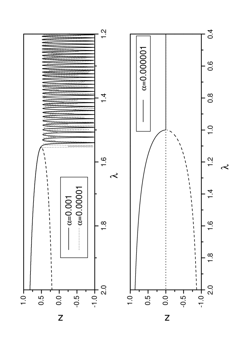
Figure 1: Time evolution of $z(t)$ initially on the elliptic fixed point $z^{\ast}(\lambda_{0})$. (a) for $\gamma=0.2,$ $\lambda_{0}=2.0.$ The solid line denotes the time evolution of $z(t)$ for $\alpha=0.001$ and dotted line for $\alpha=0.00001$. The dashed line refers to the trajectory of the hyperbolic point. (b) for $\gamma=0,$ $\lambda_{0}=2.0.$ The solid line denotes the time evolution of $z(t)$ for $\alpha=0.000001.$ The dotted line refers to the trajectory of the hyperbolic point. The dashed line refers to the trajectory of another elliptic point.

Case 1 $(\gamma\neq 0)$: For the convenience, we choose $\gamma=0.2$ and $\lambda_{0}=2$. We start at the elliptic fixed point $(z^{\ast}=z^{\ast}(\lambda_{0}),\theta^{\ast}=0)$ and $\lambda$ varies with very small $\alpha.$ At the beginning, the system follows the $z^{\ast}[\lambda(t)]$ adiabatically. But when $\lambda$ reaches $\lambda_{c}=$ $(\gamma^{2/3}+1)^{3/2},$ the adiabatic evolution is destroyed with a jump of action (the action changes to a finite value from zero suddenly) at the point $z_{c}^{\ast}\;(\approx 0.5048)$. Fig. 1(a) shows this process. Obviously, the breakdown of adiabatical condition leads to the destroy of the adiabatic evolution.

Case 2 $(\gamma=0)$: From Eq. (6) and (9), we can have two elliptic fixed points on line $\theta^{\ast}=$ $0$ for $\lambda>1$,

$$z_{\pm}^{\ast}=\pm\sqrt{1-1/\lambda^{2}},\;\theta^{\ast}=0,\;\Omega_{0}=\sqrt{\lambda(\lambda^{2}-1)},$$ (11)

and for $\lambda\leq 1,$ there is only one fixed point,

$$z^{\ast}=0,\;\theta^{\ast}=0,\;\Omega_{0}=\sqrt{1-\lambda}.$$ (12)

Obviously, for $z_{c}^{\ast}=0$ and $\lambda_{c}=1.$, $\Omega_{0}=0,$ so adiabatic condition can not be satisfied. We integrate the classical equations of the Hamiltonian system (6), with the initial condition $\lambda_{0}=2,$ $z_{0}=z_{+}^{\ast}(\lambda_{0})$, and $\theta^{\ast}(0)=0.$ Fig. 1(b) shows the time evolution of this fixed point for a very small sweeping rate $\alpha$. The final state is a very small oscillation around the fixed point $(z^{\ast}=0,\theta^{\ast}=0)$. In Fig. 2, we plot the dependency of the small oscillation amplitude $\delta$ on the sweeping rate $\alpha$. From this figure, it is clear to see that the amplitude of the small oscillation will tend to zero with the sweeping rate decreasing as a power law: $\delta=0.7\ast\alpha^{1/2}$. Therefore, for this case, the system will evolve adiabatically and keep the action not changing for all the time if the sweeping rate is small enough, even when $\lambda$ crosses the critical point $\lambda_{c}=1,$ at which $\Omega_{0}(z_{c}^{\ast})=0$, i.e., though the adiabatic condition is not satisfied when $\lambda$ crosses the point $\lambda_{c}=1$, the system is still undergoing adiabatic evolution.

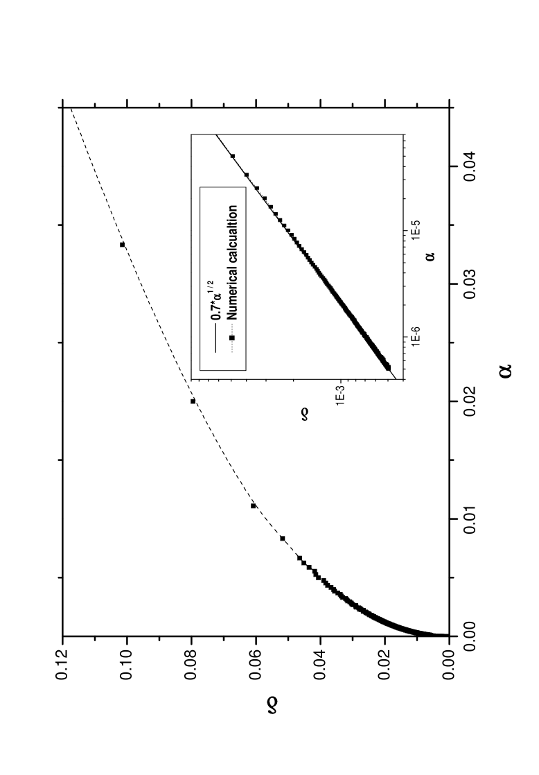
Figure 2: The dependency of the oscillation amplitude of the final state on the sweeping rate $\alpha$ for the Case 2. The initial state and parameters are the same as the Fig 1 (b) except the sweeping rate. The solid quadrangles are our numerical calculations. The solid line of insert figure is the function $0.7*\alpha^{1/2}$.

In fact, if we make the series expansion of the Hamiltonian (6) around the critical point, the system can be approximated to a double well system liufu8 . Therefore, the phenomenon of Case 2 can be illustrated by the standard double well model. Considering a particle in a double well, the system is described by the Hamiltonian $H=1/2p^{2}-1/2\mu x^{2}+1/4x^{4}.$ For $\mu>0,$ it has two stable fixed points $(x,p)=(\sqrt{\mu},0)$ and $(x,p)=(-\sqrt{\mu},0),$ and an unstable fixed point $(x,p)=(0,0);$ for $\mu<0$ it has a single stable fixed point $(x,p)=(0,0)$. At the critical point $\mu=0$, three fixed points merge into a stable fixed point. As the parameter $\mu$ varies from $+1$ to $-1$ the system goes from a double well to a single well. The stable fixed points are just the bottom of the wells, and the unstable point is just the saddle point of double well. If the particle is at the fixed point $(\sqrt{\mu},0)$ at the beginning, i.e., the particle stays at the bottom of one well. Then, let $\mu$ vary very slowly. At the critical point $\mu=0,$ the two wells merge into a single well. At this time, the bifurcation point is $(x,p)=(0,0),$ which is the bottom of the single well. So if $\mu$ varies very slowly, one can imagine that the particle will stay at the bottom of the well all the time, even when the system goes from a double well to a single one (at this time the adiabatic condition does not hold but the bifurcation point is still a stable fixed point, because the bifurcation point still corresponds to the bottom of the well).

As we have discussed in Sect. II, the breakdown of the adiabatic condition $(\Omega_{0}=0)$ corresponds to the trajectory bifurcation, i.e., the points $z_{c}^{\ast}$ is just a bifurcation point of the fixed points. The properties of the fixed points are determined by the following Jacobian

$$D=\left.\det\left(\begin{array}[]{cc}\frac{\partial\phi^{1}}{\partial z}&\frac{\partial\phi^{2}}{\partial z}\\ \frac{\partial\phi^{1}}{\partial\theta}&\frac{\partial\phi^{2}}{\partial\theta}\end{array}\right)\right|_{(z^{\ast},0)}.$$ (13)

Where $\mathbf{\phi}(z,\theta)=(\frac{\partial H}{\partial z},-\frac{\partial H}{\partial\theta})$. If the Jacobian $D\neq 0,$ the zero point (fixed point) is a regular point. But when $D=0$, the zero point is a bifurcation point.

There are two kinds of bifurcation points: limit points and branch points. The limit point satisfies that $D=0$ but $D^{1}=\left.\det\left(\begin{array}[]{cc}\frac{\partial\phi^{1}}{\partial\lambda}&\frac{\partial\phi^{2}}{\partial\lambda}\\ \frac{\partial\phi^{1}}{\partial\theta}&\frac{\partial\phi^{2}}{\partial\theta}\end{array}\right)\right|_{(z_{c}^{\ast},0)}$ $\neq 0,$ which corresponds to generation and annihilation of the fixed points.

If $D|_{(z_{c}^{\ast},0)}=D^{1}|_{(z_{c}^{\ast},0)}=0$, the point $(z_{c}^{\ast},0)$ is a branch point. The branch point corresponds to branch process of the fixed points. The directions of all branch curves are determined by the equations fu

$$A\frac{d^{2}z}{d\zeta^{2}}+2B\frac{dz}{d\zeta}+C=0,$$ (14)

or

$$C\frac{d^{2}\zeta}{dz^{2}}+2B\frac{d\zeta}{dz}+A=0,$$ (15)

where $A,$ $B,$ and $C$ are three constants. $\zeta$ corresponds to $\lambda$ or $\ \gamma$ respectively. Different solutions of the above equations correspond to different branch processes.

For the zero point $(z^{\ast},0)$, i.e., the fixed point on line $\theta^{\ast}=0,$ we can obtain $D=\left.-\sqrt{1-z^{\ast 2}}\Omega_{0}^{2}\right|_{(z^{\ast},0)}.$  Obviously, when $\Omega_{0}=0$, $D=0,$ the critical point $(z_{c}^{\ast},0)$ is a bifurcation point, at which the adiabatic condition fails.

For the case 1: We can find at the point $z_{c}^{\ast},$ the Jacobian $D=\left.-\sqrt{1-z^{2}}\Omega_{0}^{2}\right|_{(z_{c}^{\ast},0)}=0,$ but $D^{1}=\left.-s\sqrt{1-z^{2}}\right|_{(z_{c}^{\ast},0)}\neq 0.$ This point is a limit point which corresponds to annihilating of zero points. At this point, the elliptic point annihilates simultaneously with a hyperbolic point. In Fig. 1(a), the dashed lines is the trajectory of the hyperbolic point. Apparently, the elliptic point evolves adiabatically until it annihilates with the hyperbolic point at $z_{c}^{\ast}.$ After this annihilation the elliptic point turns to an ordinary closed orbit with a nonzero action, so the adiabatic evolution is destroyed. The annihilation process of the fixed points of the system (6) has also been discussed in Ref. fu2 in detail.

For the case 2: At the point $z_{c}^{\ast}=0,$ the Jacobian determinant $D=0,$ and $D^{1}=\left.-z\sqrt{1-z^{2}}\right|_{(z_{c}^{\ast},0)}=0$. This is a branch process of the fixed points. We can prove that for this case $A=C=0$, so the solutions of equations (14) and (15) give two directions: $\frac{dz}{d\lambda}=0,$ and $\frac{d\lambda}{dz}=0.$ The branch process corresponds to merging process. At this branch point, three fixed points, two elliptic points and one hyperbolic point, merge together. One can see this point in Fig. 1(b), in which the dotted line is the trajectory of the hyperbolic point, and the dashed line corresponds to the trajectory of another elliptic point. Since the total topological index is invariant, the three fixed points merge to one point with index $+1,$ i.e., merge to an elliptic point. The elliptic point evolves adiabatically until it reaches the critical point $z_{c}^{\ast},$ at which three fixed points merges to one elliptic point. Therefore, after the branch process, the elliptic point turns to a new elliptic point, the action keeps zero and the adiabatic evolution still holds.

From above discussion, we see that the adiabaticity breaks down at bifurcation points of the fixed points, but only for the limit point the adiabatic evolution is destroyed (case 1), while for this case the two fixed points annihilate. For case 2, three fixed points merge to one, because the critical point $(z_{c}^{\ast},0)$ is still a stable fixed point, the adiabatic evolution keeps with action zero.

The phenomena discussed above can occur for the adiabatic change of $\gamma$ with $\lambda$ fixed. On the other hand, the Hamiltonian (6) is invariant under the transformations $\lambda\rightarrow-\lambda,$ $\theta\rightarrow\theta+\pi,$ and $t\rightarrow-t.$ Hence, the phenomena can also be found under such transformations.

IV Conclusion

In summary, at some critical points, the adiabatic condition fails, but the adiabatic evolution may not always be broken. We find that the topological property of the critical point plays an important role for adiabatic evolution of the fixed points when the adiabatic condition does not hold. If the topological index of the critical point is $+1$ the adiabatic evolution of fixed point will not be destroyed. On the contrary, if the index of the critical point is zero or $-1$, the adiabatic evolution will be destroyed. As a paradigmatic example, we investigated the adiabatic evolution of a classical Hamiltonian system which has a number of practical interests. For this system, the adiabaticity breaks down at bifurcation points of the fixed points. But only for the limit point the adiabatic evolution is destroyed. For the branch process, the adiabatic evolution will hold, and the corrections to the adiabatic approximation tend to zero with a power law of the sweeping rate.

In general, the corrections to the adiabatic approximation are exponentially small in the adiabaticity parameter, both for quantum system and classical system book ; book1 ; book3 . It is particularly interesting that the corrections of the adiabatic approximation may be a power law (e.g., for the case 2). The power law corrections to daidabatic approximation have also been found in the nonlinear Landau-Zener tunneling wuniu . In Ref. wuniu , the authors found that when the nonlinear parameter is smaller than a critical value, the adiabatic corrections are exponentially small in the adiabatic parameter, but when the nonlinear parameter equals to the critical value, the adiabatic corrections are a power law of the adiabatic parameter. Furthermore, if the nonlinear parameter is larger than the critical value, the so-called non-zero adiabatic tunneling will occur wuniu ; add . Indeed, the cases, for which the corrects to the adiabatic approximation are not exponential law with the adiabatic parameter, correspond to the collision of fixed points.

References

- (1) L.D. Landau and E.M. Lifshitz, Quantum Mechanics (Pergamon Press, New York, 1977).
- (2) J. Moody, A. Shaper, and F. Wilczek, Adiabatic Effective Lagrangian, (in Geometric Phases in Physcis, edited by A Shapere and F. Wilczek, World Scientific Publishing Co. 1989).
- (3) L.D. Landau and E.M. Lifshitz, Mechanics (Pergamon Press, New York, 1977).
- (4) M.V. Berry, Proc. R. Soc. London A 392, 45 (1984).
- (5) D. Thouless et al., Phys. Rev. Lett. 49, 405 (1983); H. Mathur, Phys. Rev. Lett. 67, 3325 (1991).
- (6) R.G. Unanyan, N.V. Vitanov, and K. Bergmann, Phys. Rev. Lett. 87, 137902 (2001).
- (7) K. Bergmann et al., Rev. Mod. Phys. 70, 1003 (1998).
- (8) M.B. Dahan et al., Phys. Rev. Lett. 76, 4508 (1996); S.R. Wilkinson et al., Phys. Rev. Lett. 76, 4512 (1996).
- (9) S. Das, et al Phys. Rev. A bf 65, 062310 (2002); N.F. Bell, et al Phys. Rev. A 65, 042328 (2002); A.M. Childs, et al Phys. Rev. A 65, 012322 (2002); R.G. Unanyan, et al Phys. Rev. Lett. 87, 137902 (2001).
- (10) F. Dalfovo et al., Rev. Mod. Phys. 71, 463 (1999); A.J. Leggett, Rev. Mod. Phys. 73, 307 (2001); R. Dum et al., Phys. Rev. Lett. 80, 2972 (1998); Z.P. Karkuszewski, K. Sacha, and J. Zakrzewski, Phys. Rev. A63, 061601(R) (2001); T. L. Gustavson,et al, Phys. Rev. Lett. 88, 020401 (2002); J. Williams, et al Phys. Rev. A 61, 033612 (2000); Matt Mackie, et al Phys. Rev. Lett. 84, 3803 (2000); Roberto B. Diener, Biao Wu, Mark G. Raizen, and Qian Niu, Phys. Rev. Lett. 89, 070401 (2002).
- (11) Y.B. Band, B. Malomed, and M. Trippenbach, Phys. Rev. A 65, 033607 (2002); Y.B. Band and M. Trippenbach, Phys. Rev. A 65, 053602 (2002); G.J. de Valcárcel, cond-mat/0204406.
- (12) Y.S. Kivshar and B.A. Malomed, Rev. Mod. Phys. 61, 763 (1989).
- (13) R. Seydel, Practical bifurcation and stability analysis (Springer-Verlag, New York, 1994).
- (14) Li-Bin Fu, Yishi Duan, and Hong zhang, Phys. Rev. D 61, 045004 (2000); Yishi Duan, Hong zhang, and Libin Fu, Phys. Rev. E 59, 528 (1999).
- (15) Y.S. Duan, S. Li, and G.H. Yang, Nucl. Phys. B514, 705 (1998).
- (16) Jie Liu, et al., Phys. Rev. A 66, 023404 (2002); B. Wu and Q. Niu, ibid. 61, 023402 (2000).
- (17) O. Zobay and B.M. Garraway, Phys. Rev. A 61, 033603 (2000)
- (18) J.C. Eilbeck, P.S. Lomdahl, and A.C. Scott. Physica D 16, 318 (1985); V.M. Kenkre and D.K. Campbell, Phys. Rev. B 34, 4959 (1986); P.K. Datta and K. Kundu, ibid. 53, 14929 (1996).
- (19) M.R. Andrews, C.G. Townsend, H.-J. Miesner, D.S. Durfee, D.M. Kurn, and W. Ketterle, Science 275, 637 (1997).
- (20) A. Smerzi, S. Fantoni, S. Giovanazzi, and S.R. Shenoy, Phys. Rev. Lett. 79, 4950 (1997); G.J. Milburn et al., Phys. Rev. A 55, 4318 (1997).
- (21) M.O. Mewes, M.R. Andrews, D.M. Kurn, D.S. Durfee, C.G. Townsend, and W. Ketterle, Phys. Rev. Lett. 78, 582 (1997).
- (22) M.H. Anderson, M.R. Matthews, C.W. Wieman, and E.A. Cornell, Science 269, 198 (1995).
- (23) Dae-II Choi, and Qian Niu, Phys. Rev. Lett. 82, 2022 (1999).
- (24) C. Lee, W. Hai, L. Shi, and K. Gao, Phys. Rev. A 69, 033611 (2004); C. Lee, W. Hai, X. Luo, L. Shi, and K. Gao. ibid. 68, 053614 (2003); W. Hai, C. Lee, G. Chong, and L. Shi, Phys. Rev. E 66, 026202 (2002); C. Lee, et al., Phys. Rev. A 64, 053604 (2001).
- (25) Li-Bin Fu, Jie Liu, and Shi-Gang Chen, Phys. Lett. A 298, 388 (2002).
- (26) J. Liu, B. Wu, L. Fu, R.B. Diener, and Q. Niu, Phys. Rev. B 65, 224401 (2002).
- (27) Li-Bin Fu, Jie Liu, Shi-Gang Chen, and Yishi Duan, J. Phys. A: Math. Gen. 35, L181 (2002).