Parameterizing Quasiperiodicity: Generalized Poisson Summation and Its Application to Modified-Fibonacci Antenna Arrays

Abstract

The fairly recent discovery of “quasicrystals”, whose X-ray diffraction patterns reveal certain peculiar features which do not conform with spatial periodicity, has motivated studies of the wave-dynamical implications of “aperiodic order”. Within the context of the radiation properties of antenna arrays, an instructive novel (canonical) example of wave interactions with quasiperiodic order is illustrated here for one-dimensional (1-D) array configurations based on the “modified-Fibonacci” sequence, with utilization of a two-scale generalization of the standard Poisson summation formula for periodic arrays. This allows for a “quasi-Floquet” analytic parameterization of the radiated field, which provides instructive insights into some of the basic wave mechanisms associated with quasiperiodic order, highlighting similarities and differences with the periodic case. Examples are shown for quasiperiodic infinite and spatially-truncated arrays, with brief discussion of computational issues and potential applications.

1 Introduction

The recent discovery (1984) of “quasicrystals”, i.e., certain metallic alloys whose X-ray diffraction patterns contain bright spots displaying symmetries (e.g., 5-fold) which are incompatible with spatial periodicity [1], [2], has stimulated a growing interest in the study of aperiodic order and its wave-dynamical properties.

In electromagnetics (EM) engineering, use of random or deterministic aperiodic geometries has been customary within the framework of antenna array thinning [3]–[5], whereas multiperiod configurations have recently been proposed for optimizing the passband/stopband characteristics of frequency selective surfaces [6] and photonic bandgap (PBG) devices [7]. In [8], we explored the radiation properties of two-dimensional (2-D) antenna arrays based on the concept of “aperiodic tiling” [9], [10], which had previously found interesting applications in the field of PBG devices (see the brief summary and references in [8]).

In this paper, we turn our attention to the radiation properties of a different category of aperiodic structures consisting of two-scale Fibonacci-type sequences [11]. Materials exhibiting this type of aperiodic order, technically called “quasiperiodicity” (see the definition in Sec. 2.2), were first fabricated in 1985 as GaAs-AlAs heterostructures (1-D multilayers) [12]; their technical classification as “quasicrystals” is still debated [13]. The wave-dynamical properties of 1-D and 2-D Fibonacci-type structures have been widely investigated, theoretically and experimentally, in quantum mechanics, acoustics and EM (see [14]–[26] for a sparse sampling). Particularly interesting outcomes concern the self-similar fractal (Cantor-type) nature of the eigenspectra [14], [16], [20], and the possible presence of bandgaps [19], [21], omnidirectional reflection properties [22], [25], and localization phenomena [14], [18], [23].

Here, we concentrate on the study of the radiation properties of a simple class of 1-D antenna arrays based on the so-called “modified-Fibonacci” sequence. This novel prototype array configuration appears particularly well suited to exploration of some basic characteristics of wave interactions with quasiperiodic order. First, this array model is amenable to analytic parameterization via a generalized Poisson summation formula, by exploiting some recent results in [27] (this paper is easily accessible through the web). Note that, in principle, one can derive generalized Poisson summation formulas that accommodate a variety of “nonperiodicity scales” (see, e.g., [28]). Here, we consider only two scales, $d_{1}$ and $d_{2}$. This opens up the possibility of extending the Floquet-based parameterization of infinite and semi-infinite time-harmonic periodic arrays in [29], [30] to the case of two-scale quasiperiodic arrays. Next, the inherent degree of freedom in the choice of the ratio between the two scales can be used to study the “transition” from periodic ($d_{1}=d_{2}$) to quasiperiodic ($d_{1}\neq d_{2}$) order, so as to better understand the quasiperiodicity-induced footprints in the wave dynamics. Finally, although the main focus of this preliminary investigation is on wave-dynamical phenomenologies, computational and applicational issues for a test example are briefly addressed as well, including possible exploitation of the two-scale degree of freedom for pattern control in practical applications.

The paper is organized as follows. In Section 2, the problem geometry is described, and the modified-Fibonacci sequence is introduced together with general aspects of quasiperiodicity. In Section 3, the generalized Poisson summation formula for modified-Fibonacci arrays is introduced, and its similarities and differences with the periodic case are discussed. In Section 4, a “quasi-Floquet” (QF) parameterization of the radiated field for infinite and semi-infinite modified-Fibonacci arrays is derived, paralleling [29], [30]. Numerical results and potential applications are illustrated in Section 5, followed by brief concluding remarks in Section 6.

2 Background and Problem Formulation

2.1 Geometry

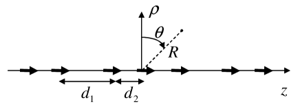
Figure 1: Problem schematic: An infinite (or semi-infinite) phased line array of $z$-directed electric dipoles is considered. The dipole distribution $z_{m}$, which features only two possible inter-element spacings $d_{1}$ and $d_{2}\leq d_{1}$, is chosen according to the modified-Fibonacci sequence in (5). Also shown are the $(z,\rho)$ and $(R,\theta)$ coordinate systems utilized.

Referring to the geometry depicted in Fig. 1, we begin with an infinite phased line array of $z$-directed electric dipoles, subject to uniform unit-amplitude time-harmonic $\exp(j\omega t)$ excitation, described by the current distribution

$$f(z)=\sum_{m=-\infty}^{\infty}\delta(z-z_{m})\exp\left(-j\eta k_{0}z_{m}\right),$$ (1)

where $k_{0}=\omega\sqrt{\epsilon_{0}\mu_{0}}=2\pi/\lambda_{0}$ is the free-space wavenumber (with $\lambda_{0}$ being the wavelength), and $-1\leq\eta\leq 1$ describes the inter-element phasing. The dipole sequence $\left\{z_{m}\right\}_{m=-\infty}^{\infty}$, which is restricted to two possible inter-element spacings $d_{1}$ and $d_{2}\leq d_{1}$ (see Fig. 1), is chosen according to the modified-Fibonacci rule, whose properties are summarized below. Spatial truncation effects will be discussed in Sec. 4.2.

2.2 Modified-Fibonacci Sequence: An Example of
Quasiperiodic Order

The Fibonacci sequence [11], introduced in 1202 by the Italian mathematician Leonardo da Pisa (Fibonacci) (ca. 1170–ca. 1240), in connection with a model for rabbit breeding, is probably the earliest and most thoroughly investigated deterministic aperiodic sequence. Since then, it has found applications in many different fields, owing to its intimate relation with one of the most pervasive mathematical entities, the Golden Mean [11]. In its simplest version, the Fibonacci sequence can be generated from a two-symbol alphabet ${\cal A}=\left\{a,b\right\}$, by iteratively applying the substitution rules

$$a\rightarrow ab,~{}~{}b\rightarrow a,$$ (2)

so as to construct a sequence of symbolic strings $s_{n}$

$$b\Rightarrow a\Rightarrow ab\Rightarrow aba\Rightarrow abaab\Rightarrow abaababa\Rightarrow abaababaabaab\cdots$$ (3)

Note that the string at each iteration is obtained as the concatenation of the two preceding ones ($s_{n}=s_{n-1}\cup s_{n-2}$). The process can be iterated ad infinitum, yielding an infinite sequence of “$a$” and “$b$” symbols which seems to display no apparent regularity, but actually hides a wealth of interesting properties (see [11] for details). For instance, in the limit of an infinite sequence, it can be shown that the ratio between the numbers of “$a$” and “$b$” symbols ($N_{a}$ and $N_{b}$, respectively) approaches the Golden Mean $\tau=(1+\sqrt{5})/2$ [11],

$$\lim_{N\rightarrow\infty}\frac{N_{a}}{N_{b}}=\tau=\frac{1+\sqrt{5}}{2},~{}~{}~{}N_{a}+N_{b}=N.$$ (4)

In connection with the antenna array problem of interest here, there are several ways of embedding the above-introduced Fibonacci-type aperiodic sequence. One possibility would be keeping the geometry periodic (i.e., uniform inter-element spacing) and associating with the “$a$” and “$b$” symbols in the Fibonacci sequence two possible current amplitudes. Another possibility, pursued in this investigation, assumes uniform excitation and associates the “$a$” and “$b$” symbols with two possible inter-element spacings, $d_{1}$ and $d_{2}\leq d_{1}$, respectively (see Fig. 1). Accordingly, the dipole positions $z_{m}$ in (1) can be obtained from the symbolic strings in (3) or, in an equivalent and more direct fashion, via [27]

$$z_{m}=d_{1}\left\|\frac{m}{\tau}\right\|+d_{2}\left(m-\left\|\frac{m}{\tau}\right\|\right),$$ (5)

where $\left\|\cdot\right\|$ denotes the nearest-integer function,

$$\left\|x\right\|=\left\{\begin{array}[]{ll}m,~{}~{}~{}~{}~{}~{}~{}~{}~{}~{}~{}~{}m\leq x<m+\frac{1}{2},\\ m+1,~{}~{}~{}~{}~{}~{}m+\frac{1}{2}\leq x\leq m+1.\end{array}\right.$$ (6)

Following [27], the particular case $d_{2}=d_{1}/\tau$ in (5) will be referred to as “standard Fibonacci”. The general case, in which the scale ratio $\nu=d_{2}/d_{1}$ is left as a degree of freedom, will be referred to as “modified Fibonacci”, and represents one of the simplest extensions of the Fibonacci sequence. The reader is referred to [28], [31], [32] for other examples of possible extensions/generalizations.

Note that the modified-Fibonacci sequence in (5) includes as a limit the periodic case ($d_{1}=d_{2}$). It can be proved that, with the exception of this degenerate case, the sequence in (5) and the corresponding dipole distribution in (1) display a “quasiperiodic” character, which represents one of the most common and best known forms of aperiodic order. The concept of quasiperiodicity stems from the theory of “almost-periodic” functions developed by H. Bohr during the 1920s [33], [34]. In essence, a quasiperiodic function can be uniformly approximated by a generalized Fourier series containing a countable infinity of pairwise incommensurate frequencies generated from a finite-dimensional basis (see [33], [34] for more details).

It follows from (4) that, in the infinite-sequence limit, the average inter-element spacing $d_{av}$ is [27]

$$d_{av}=\frac{\tau d_{1}+d_{2}}{1+\tau}.$$ (7)

Anticipating the analytic derivations and parametric analysis in Secs. 3 and 4, it is expedient to parameterize the sequence in (5) in terms of the average spacing $d_{av}$ in (7) and the scale ratio $\nu=d_{2}/d_{1}$, rewriting $d_{1}$ and $d_{2}$ as

$$d_{1}=\frac{(1+\tau)}{(\nu+\tau)}d_{av},~{}~{}~{}d_{2}=\nu d_{1},~{}~{}0<\nu\leq 1.$$ (8)

The modified-Fibonacci sequence in (5) admits an instructive alternative interpretation in terms of a “cut-and-project” graphic construction [27], as illustrated in Fig. 2. Cut-and-project schemes are systematic tools for generating quasiperiodic sets via projection from higher-dimensional periodic lattices (see [10] for details). In our case, one starts from a 2-D square lattice of side $d_{0}=d_{1}\sqrt{1+\nu^{2}}$ traversed by a straight line with slope $\tan\phi_{0}=1/\tau$. Those lattice points whose “Voronoï cell” [10] (light-shaded square cell of side $d_{0}$ centered around the point, in Fig. 2) is crossed by the line (or, equivalently, those falling within the rectangular window of size $h=d_{0}(1+\tau)/\sqrt{2+\tau}$ centered around the line, in Fig. 2) are orthogonally projected onto another straight line ($z$-axis in Fig. 2) with slope $\tan\phi=\nu$ to yield the desired modified-Fibonacci sequence in (5). For the standard-Fibonacci sequence ($\nu=1/\tau$), the two lines coincide ($\phi=\phi_{0}$) and the above scheme becomes equivalent to the canonical cut-and-project scheme described in [10].

3 Generalized Poisson Summation Formula

For periodic structures, Floquet theory provides a rigorous and powerful framework for spectral- or spatial-domain analytic and numerical analysis. In this connection, the Poisson summation formula [35] can be utilized to systematically recast field observables as superpositions of either individual or collective contributions. Problem-matched extensions have also been developed to accommodate typical departures from perfect periodicity in realistic structures, such as truncation (finiteness) and smooth perturbations in the spatial period as well as in the excitation (tapering) [36]–[39].

Considering the degenerate periodic limiting case ($d_{1}=d_{2}=d$, i.e., $z_{m}=md$) of the modified-Fibonacci sequence in (5), the corresponding periodic limit $f^{(per)}$ of the current distribution in (1) can be recast, via the standard Poisson summation formula [35], as

$$f^{(per)}(z)=\sum_{m=-\infty}^{\infty}\delta(z-md)\exp\left(-j\eta k_{0}md\right)$$ (9a)

$$=\frac{1}{d}\sum_{q=-\infty}^{\infty}\exp\left(-jk_{zq}z\right),~{}~{}k_{zq}=k_{0}\eta+\frac{2\pi q}{d}.$$ (9b)

The $m$-indexed individual dipole contributions in (9a) are thereby recast into the infinite superposition of linearly smoothly-phased $q$-indexed equivalent line source distributions in (9b). Remarkably, a similar re-parameterization is always possible for the general (i.e., quasiperiodic) case of the modified-Fibonacci sequence in (5), since it can be shown that the spatial Fourier transform (plane-wave spectrum) of (1) can be written as [27] (see also the Appendix)

$${\hat{F}}(k_{z}) = \int_{-\infty}^{\infty}f(z)\exp(jk_{z}z)dz$$ (10a)

$$= \sum_{m=-\infty}^{\infty}\exp(jk_{z}z_{m})\exp\left(-j\eta k_{0}z_{m}\right)$$

$$= \frac{2\pi}{d_{av}}\sum_{q_{1},q_{2}=-\infty}^{\infty}S_{q_{1}q_{2}}\delta(k_{z}-k_{zq_{1}q_{2}}),$$ (10b)

where $d_{av}$ is defined in (7), and the amplitude coefficients $S_{q_{1}q_{2}}$ and the spatial frequencies $k_{zq_{1}q_{2}}$ are given by

$$S_{q_{1}q_{2}} = \frac{\sin W_{q_{1}q_{2}}}{W_{q_{1}q_{2}}},$$

$$W_{q_{1}q_{2}} = \frac{\pi}{d_{av}}\left(q_{1}d_{1}-q_{2}d_{2}\right)=\frac{\pi(1+\tau)(q_{1}-q_{2}\nu)}{\nu+\tau},$$ (11)

$$k_{zq_{1}q_{2}}=k_{0}\eta+\alpha_{q_{1}q_{2}},~{}~{}\alpha_{q_{1}q_{2}}=\frac{2\pi}{d_{av}}\frac{(q_{1}+q_{2}\tau)}{(\tau+1)}.$$ (12)

It then follows via straightforward inverse Fourier transform of (10b) that

$$f(z)=\frac{1}{d_{av}}\sum_{q_{1},q_{2}=-\infty}^{\infty}S_{q_{1}q_{2}}\exp\left(-jk_{zq_{1}q_{2}}z\right).$$ (13)

Equation (13) thus represents a generalization of the standard Poisson summation formula for periodic arrays in (9) to the more general quasiperiodic modified-Fibonacci array in (5), and will accordingly be referred to as generalized Poisson summation formula. It is readily verified that for the special case of periodic arrays ($d_{1}=d_{2}=d$, i.e., $\nu=1$), one obtains

$$d_{av}=d,~{}~{}W_{q_{1}q_{2}}=(q_{1}-q_{2})\pi,~{}~{}S_{q_{1}q_{2}}=\delta_{q_{1}q_{2}},$$ (14)

with $\delta_{q_{1}q_{2}}$ denoting the Kronecker delta, and thus (13) reduces to the standard Poisson summation formula in (9b).

A few observations are in order to highlight similarities and differences between (13) and (9). Similar to (9), the individual dipole contributions in (5) are recast via (13) as a superposition of collective contributions arising from linearly smoothly-phased equivalent line source distributions. However, at variance with the $q$-indexed single infinity of equispaced spatial frequencies in (9b), the generalized Poisson summation formula in (13) entails a $(q_{1},q_{2})$-indexed double infinity of generally pairwise-incommensurate spatial frequencies. This could be expected recalling the definition of the quasiperiodic functions given in Sec. 2.2. Note that the spatial frequencies $k_{zq_{1}q_{2}}$ in (12) depend on the average inter-element spacing $d_{av}$, but are independent of the scale ratio $\nu=d_{2}/d_{1}$. The dependence on $\nu$ shows up (via $W_{q_{1}q_{2}}$) in the amplitude coefficients $S_{q_{1}q_{2}}$ in (11), which are not constant as for the periodic case in (9b). It is worth pointing out that such dependence is smooth, and consequently no abrupt transition occurs when $\nu$ is varied between rational and irrational values, i.e., going from commensurate to incommensurate scales $d_{1}$ and $d_{2}$. However, for case of commensurate scales,

$$\nu=\frac{d_{2}}{d_{1}}=\frac{p_{1}}{p_{2}},~{}~{}p_{1},p_{2}\in{\mathbb{N}},$$ (15)

one can readily verify that

$$k_{z(q_{1}+Mp_{1})(q_{2}+Mp_{2})} = k_{zq_{1}q_{2}}+M\left(\frac{2\pi}{d_{1}}p_{2}\right),$$

$$W_{(q_{1}+Mp_{1})(q_{2}+Mp_{2})} = W_{q_{1}q_{2}},~{}~{}M\in{\mathbb{Z}},$$ (16)

and thus the array spectrum in (10b) is periodic with period $2\pi p_{2}/d_{1}$. It can be verified that the opposite implication is also true, and thus the spectrum is periodic if and only if the scales $d_{1}$ and $d_{2}$ are commensurate, although the array remains aperiodic in physical space [27].

4 Radiated Field

In order to further explore possible similarities and differences between the wave phenomenologies associated with periodicity and quasiperiodicity, it is instructive to consider the radiated fields. To this end, in what follows, we extend the Floquet-based frequency-domain analysis in [29], [30], for infinite and semi-infinite periodic phased arrays of dipoles, to the quasiperiodic modified-Fibonacci case. As in [29], [30], attention is restricted to the $z$-directed vector potential ${\bf A}({\bf r})=A({\bf r}){\bf u}_{z}$, with ${\bf r}\equiv(z,\rho)$ and with ${\bf u}_{z}$ denoting a $z$-directed unit vector, from which all field quantities of interest can be computed. Whenever applicable, partial results from [29], [30] are recalled and used, without going into the details of the technical derivations.

4.1 Infinite Arrays

For infinite arrays, proceding analogous to [29], the generalized Poisson summation formula in (13) can be used to recast the element-by-element (spherical wave) synthesis of the field potential,

$$A({\bf r}) = \int_{-\infty}^{\infty}f(z^{\prime})\frac{\exp\left(-jk_{0}R\right)}{4\pi R}dz^{\prime}=\sum_{m=-\infty}^{\infty}A_{m}({\bf r})$$ (17)

$$= \sum_{m=-\infty}^{\infty}\frac{\exp\left(-jk_{0}R_{m}\right)}{4\pi R_{m}}\exp\left(-jk_{0}\eta z_{m}\right),$$

where $R=\sqrt{\rho^{2}+(z-z^{\prime})^{2}}$ and $R_{m}=\sqrt{\rho^{2}+(z-z_{m})^{2}}$, in terms of a “quasi-Floquet” (QF) representation

$$A({\bf r})=\sum_{q_{1},q_{2}=-\infty}^{\infty}S_{q_{1}q_{2}}A^{QF}_{q_{1}q_{2}}({\bf r}),$$ (18)

$$A^{QF}_{q_{1}q_{2}}({\bf r}) = \frac{1}{d_{av}}\int_{-\infty}^{\infty}\frac{\exp\left(-jk_{0}R\right)}{4\pi R}\exp\left(-jk_{zq_{1}q_{2}}z^{\prime}\right)dz^{\prime}$$ (19)

$$= \frac{\exp\left(-jk_{zq_{1}q_{2}}z\right)}{4jd_{av}}\mbox{H}_{0}^{(2)}\left(k_{\rho q_{1}q_{2}}\rho\right).$$

In (19), $\mbox{H}_{0}^{(2)}$ denotes the zeroth-order Hankel function of the second kind (line-source Green’s function), and $k_{\rho q_{1}q_{2}}=\sqrt{k_{0}^{2}-k^{2}_{zq_{1}q_{2}}}$, $\mbox{Im}\left(k_{\rho q_{1}q_{2}}\right)\leq 0$ denote the QF wave radial wavenumbers related to the $z$-domain wavenumbers $k_{zq_{1}q_{2}}$ in (12). Recalling the asymptotic ($|k_{\rho q_{1}q_{2}}\rho|\rightarrow\infty$) expansion of the Hankel function, one obtains

$$A^{QF}_{q_{1}q_{2}}({\bf r}) \sim\frac{1}{d_{av}\sqrt{4\pi k_{\rho q_{1}q_{2}}\rho}}$$ (20)

$$\times \exp\left[-j\left(k_{\rho q_{1}q_{2}}\rho+k_{zq_{1}q_{2}}z+\frac{\pi}{4}\right)\right],$$

from which it is recognized that

$$\left|k_{zq_{1}q_{2}}\right|<k_{0},~{}~{}~{}q_{2}\lessgtr-\frac{q_{1}}{\tau}\pm\left(\frac{d_{av}}{\lambda_{0}}\right)\frac{\left(1\mp\eta\right)\left(1+\tau\right)}{\tau},$$ (21)

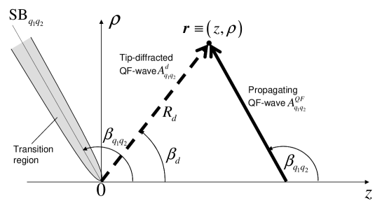
Figure 3: Quasi-Floquet (QF) wave phenomenologies for the infinite and semi-infinite array (planar cut through conical wavefields). For the infinite array, the wavefield away from the array axis is synthesized in terms of propagating QF waves $A^{QF}_{q_{1}q_{2}}$ (heavy solid arrow) arriving from direction $\beta_{q_{1}q_{2}}$ in (22). For the semi-infinite array, the region of validity of each propagating QF wave is limited by a conical shadow boundary SB${}_{q_{1}q_{2}}$ with the same angle $\beta_{q_{1}q_{2}}$. A spherical tip-diffracted QF wave $A^{d}_{q_{1}q_{2}}$ (dashed arrow) arriving from direction $\beta_{d}$ ensures, via the transition function in (27), continuity of the wavefield across the parabolic transition region (gray shading) surrounding the shadow boundary cone.

corresponds to radially-propagating QF waves, whereas $|k_{zq_{1}q_{2}}|>k_{0}$ corresponds to radially-evanescent QF waves. Accordingly, sufficiently far from the array axis, the potential field in (18) will be synthesized in terms of conical propagating QF waves (heavy solid arrow in Fig. 3), with arrival directions

$$\beta_{q_{1}q_{2}}=\arccos\left(\frac{k_{zq_{1}q_{2}}}{k_{0}}\right).$$ (22)

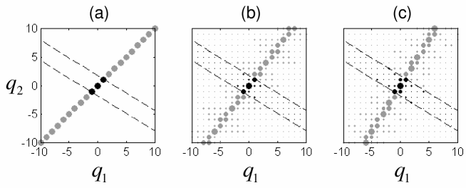
Figure 4: Modified-Fibonacci array with $d_{av}=1.1\lambda_{0},\eta=0$, and various values of the scale ratio $\nu=d_{2}/d_{1}$. ($q_{1},q_{2}$)-plane mapping of propagating (dark dots) and evanescent (light dots) amplitude coefficients $S_{q_{1}q_{2}}$ in (11). Only $|q_{1}|,|q_{2}|\leq 10$ spatial frequencies are considered, with dot size proportional to coefficient amplitude. The two oblique dashed lines delimit the propagating spectral range in (21). (a): $\nu=1$ (periodic); (b): $\nu=0.75$; (c): $\nu=1/\tau$ (standard-Fibonacci).

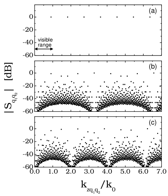
Figure 5: As in Fig. 4, but $|S_{q_{1}q_{2}}|$ vs. $k_{zq_{1}q_{2}}$, for $|q_{1}|,|q_{2}|\leq 50$ and $k_{zq_{1}q_{2}}\leq 7k_{0}$. Due to symmetry, only positive spatial frequencies are shown.

In the $(q_{1},q_{2})$-plane, the propagating spectral range in (21) is mapped into an infinite strip, thus indicating the general presence of an infinite number of propagating QF waves. This is illustrated in Fig. 4, for a nonphased ($\eta=0$) array with $d_{av}=1.1\lambda_{0}$ and various values of the scale ratio $\nu=d_{2}/d_{1}$. Also shown, for comparison, is the periodic case (Fig. 4(a)), which entails a finite number of propagating Floquet waves. In the general quasiperiodic case, it is observed that the propagating spectral range is vastly populated, irrespective of the commensurate (Fig. 4(b)) or incommensurate (Fig. 4(c)) character of the scales $d_{1}$ and $d_{2}$. However, it follows from (11) that moving toward large values of $q_{1},q_{2}$ (with opposite sign), the amplitude coefficients $S_{q_{1}q_{2}}$ decay non-monotonically as $\sim(q_{1}-q_{2}\nu)^{-1}$. For a better quantitative understanding, Fig. 5 shows the direct mapping $S_{q_{1}q_{2}}$ vs. $k_{zq_{1}q_{2}}$ for the same array configurations as in Fig. 4 and $|q_{1}|,|q_{2}|\leq 50$. Apart from the trivial periodic case (Fig. 5(a)), one observes highly-populated spectra, which display perfect periodicity in the case of commensurate scales (Fig. 5(b)) and only some loose repetitiveness otherwise (Fig. 5(c)). In both cases, a vast majority of the spatial frequencies have amplitude coefficients significantly smaller ($\lesssim-20$dB) than the dominant ones.

4.2 Truncation Effects: Semi-Infinite Arrays

Capitalizing on some analogies with the problem expounded in [30], we have also studied truncation-induced diffraction effects. For the semi-infinite ($m\geq 0$) version of the array in (1), one obtains a truncated QF wave synthesis,

$$A({\bf r}) = \sum_{m=0}^{\infty}A_{m}({\bf r})$$ (23)

$$= \sum_{m=0}^{\infty}\frac{\exp\left(-jk_{0}R_{m}\right)}{4\pi R_{m}}\exp\left(-jk_{0}\eta z_{m}\right)$$

$$= \frac{A_{0}({\bf r})}{2}+\sum_{q_{1},q_{2}=-\infty}^{\infty}S_{q_{1}q_{2}}A^{T}_{q_{1}q_{2}}({\bf r}),$$

where $A^{T}_{q_{1}q_{2}}$ are truncated QF wave propagators,

$$A^{T}_{q_{1}q_{2}}({\bf r}) = \frac{1}{d_{av}}\int_{0}^{\infty}\frac{\exp\left(-jk_{0}R\right)}{4\pi R}\exp\left(-jk_{zq_{1}q_{2}}z^{\prime}\right)dz^{\prime}$$ (24)

$$= \frac{\exp\left(-jk_{zq_{1}q_{2}}z\right)}{8\pi d_{av}}\int_{-\infty}^{\infty}\frac{\mbox{H}_{0}^{(2)}\left(k_{\rho q_{1}q_{2}}\rho\right)}{k_{z}-k_{zq_{1}q_{2}}}dk_{z}.$$

Exploiting the uniform high-frequency asymptotic approximation given in Eqs. (28)–(35) of [30] for the spectral integral in (24), one obtains

$$A^{T}_{q_{1}q_{2}}({\bf r})\sim A^{QF}_{q_{1}q_{2}}({\bf r})U\left(\beta_{q_{1}q_{2}}^{SB}-\beta_{d}\right)+A^{d}_{q_{1}q_{2}}({\bf r}).$$ (25)

In (25), $A^{QF}_{q_{1}q_{2}}$ is the QF wave propagator in (20), $U$ denotes the Heaviside unit-step function, $\beta^{SB}_{q_{1}q_{2}}$ delimits the shadow-boundary of each QF wave (for propagating QF waves, $\beta_{q_{1}q_{2}}^{SB}=\beta_{q_{1}q_{2}}$). Moreover, $A^{d}_{q_{1}q_{2}}$ represents the diffracted QF wave emanating from the array tip,

$$A^{d}_{q_{1}q_{2}}({\bf r})\sim\frac{\exp\left(-jk_{0}R_{d}\right)}{j4\pi d_{av}k_{0}R_{d}}\frac{F(\gamma^{2}_{q_{1}q_{2}})}{\left(\cos\beta_{q_{1}q_{2}}-\cos\beta_{d}\right)},$$ (26)

where $R_{d}=\sqrt{\rho^{2}+z^{2}}$, $\beta_{d}=\arctan(\rho/z)$, $\gamma_{q_{1}q_{2}}=\sqrt{2k_{0}R_{d}}\sin[(\beta_{q_{1}q_{2}}-\beta_{d})/2]$, and $F$ denotes the standard transition function of the uniform theory of diffraction (UTD),

$$F(x)=2j\sqrt{x}\exp(jx)\int_{\sqrt{x}}^{\infty}\exp\left(-j\xi^{2}\right)d\xi,$$

$$-\frac{3}{2}\pi<\mbox{arg}(x)\leq\frac{\pi}{2}.$$ (27)

The wave phenomenologies are illustrated in Fig. 3, for the case of propagating ($|k_{zq_{1}q_{2}}|<k_{0}$) QF waves. The region of validity of each QF wave $A^{QF}_{q_{1}q_{2}}$ (heavy arrow in Fig. 3) arriving from direction $\beta_{q_{1}q_{2}}$ is now limited by a conical shadow boundary. The spherical tip-diffracted QF wave $A^{d}_{q_{1}q_{2}}$ (dashed arrow in Fig. 3) arriving from direction $\beta_{d}$ ensures, via the transition function in (27), continuity of the wavefield across the parabolic transition region (gray shading in Fig. 3) surrounding the shadow boundary cone.

Note that evanescent ($|k_{zq_{1}q_{2}}|>k_{0}$) QF waves yield negligible contributions at observation points far from the array axis, but they excite propagating diffracted fields that need to be taken into account. As in [30] (see the discussion after Eq. (35) there), these contributions are approximated via nonuniform asymptotics ($F\approx 1$ in (26)). We point out that, at variance with the periodic array case (cf. Eq. (36) in [30]), it is not possible here to recast the total spherical wave diffracted field in a more manageable form.

5 Results and Potential Applications

Although our main interest in this preliminary investigation is focused on wave-dynamical phenomenologies associated with radiation from quasiperiodic antenna arrays, we briefly discuss some computational and applicational aspects with the hope of providing further insights. We stress that no attempt has been made at this stage to devise optimal computational schemes, nor do we deal with actual fabrication-oriented issues (feeding, matching, inter-element coupling, etc.).

5.1 Numerical Results

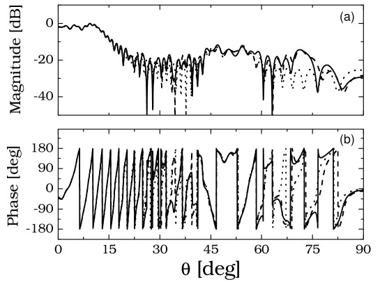
Figure 6: $101$-element standard-Fibonacci ($\nu=1/\tau$) array with $d_{av}=0.5\lambda_{0}$ and $\eta=0$. Near-zone ($R=100\lambda_{0}$) normalized potential field scan. —– Reference solution (element-by-element summation); $\cdots\cdots$ QF synthesis retaining $N_{p}=3$ dominant propagating waves (selected within $|q_{1}|,|q_{2}|\leq 50$); - - - QF synthesis retaining $N_{p}=9$ dominant propagating QF waves. Due to symmetry, only positive angles are shown.

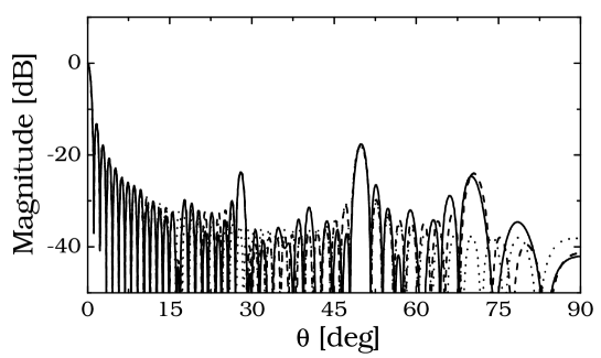
Figure 7: As in Fig. 6, but far-field pattern.

From a computational viewpoint, the actual utility of the QF syntheses in Sec. 4 (double summations involving an infinite number of propagating waves) might appear questionable as compared with brute-force element-by-element synthesis. However, as observed in Sec. 4.1 (see also Fig. 5), under appropriate conditions, a large number of propagating QF waves could be weakly excited, thus suggesting the possibility, yet to be explored, of devising effective truncation schemes. Here, we try to quantify some of these aspects via numerical examples. We begin by considering a 101-element nonphased standard-Fibonacci array ($\eta=0$, $\nu=1/\tau$, $|m|\leq 50$ in (1)). The truncated QF synthesis developed in Sec. 4.2 for a semi-infinite array can readily be exploited here by expressing the finite array interval as the difference between two overlapping semi-infinite intervals. Figure 6 shows the near-field ($R=100\lambda_{0}$) QF synthesis results for $d_{av}=0.5\lambda_{0}$, using the crudest possible truncation criterion based on retaining $N_{p}$ dominant propagating QF waves in (23). Also shown, as a reference solution, is the element-by-element synthesis in (17) (with $|m|\leq 50$). It is observed that the QF synthesis with $N_{p}=9$ propagating waves provides reasonably good agreement, and even $N_{p}=3$ is still capable of fleshing out most of the wavefield structure. Similar statements can be made for the far-field pattern in Fig. 7. In order to better quantify the accuracy, and address convergence issues, we have computed the r.m.s. error

$$\Delta A(R)=\sqrt{\frac{\int_{-\pi/2}^{\pi/2}\left|A^{RS}(R,\theta)-A^{QF}(R,\theta)\right|^{2}d\theta}{\int_{-\pi/2}^{\pi/2}\left|A^{RS}(R,\theta)\right|^{2}d\theta}},$$ (28)

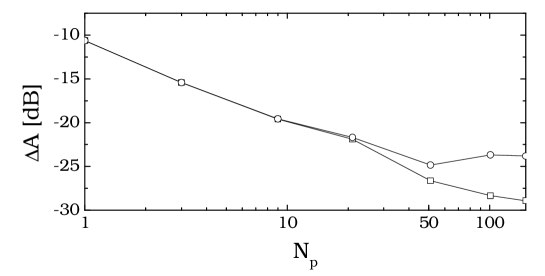
Figure 8: Parameters as in Fig. 6, but r.m.s. error $\Delta A$ in (28) vs. number $N_{p}$ of propagating waves retained in the near field ($R=100\lambda_{0}$) QF synthesis. Circular bullets: No evanescent diffracted waves retained. Square bullets: $N_{e}=N_{p}$ evanescent diffracted waves retained. Results for the far-field are practically identical.

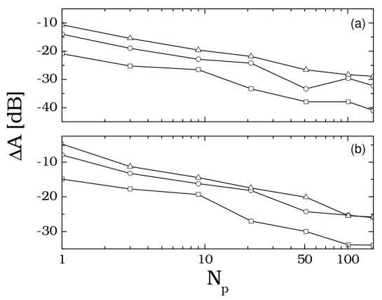
Figure 9: As in Fig. 8, with $R=100\lambda_{0}$, $N_{e}=N_{p}$, and various values of scale ratio $\nu=d_{2}/d_{1}$ and average spacing $d_{av}$. (a): $d_{av}=0.5\lambda_{0}$. (b): $d_{av}=0.75\lambda_{0}$. Square bullets: $\nu=0.9$. Circular bullets: $\nu=0.75$. Triangular bullets: $\nu=1/\tau$.

where the subscripts “^RS” and “^QF” denote the reference solution and the QF synthesis, respectively. Figure 8 shows the error behavior vs. the number $N_{p}$ of dominant propagating QF waves retained, for near-field synthesis (results for the far-field are practically identical). Also shown, for comparison, are results obtained by retaining a number $N_{e}=N_{p}$ of dominant evanescent QF diffracted waves. It is observed that a moderate number ($\sim 10$) of QF waves is capable of providing acceptable accuracy ($\Delta A\sim-20$dB). The contribution of $N_{e}$ retained evanescent QF diffracted waves is practically negligible for $N_{e}\lesssim 20$, but can give observable improvements at larger $N_{e}$-values. Intuitively, one would expect the convergence behavior to improve in the presence of weaker aperiodicity ($\nu\approx 1$) and smaller average inter-element spacing, and viceversa. This is confirmed by the results shown in Fig. 9, for two values of the inter-element spacing ($d_{av}=0.5\lambda_{0}$ and $0.75\lambda_{0}$) and three values of the scale ratio ($\nu=0.9,0.75$ and $1/\tau$).

To sum up, the above results seem to indicate that moderate-size QF syntheses, truncated by using even crude criteria, can still be capable of capturing the dominant features of the relevant wave dynamics. However, besides the computational convenience, which can become questionable if highly accurate results are needed, the QF parameterization can offer valuable insights for judicious exploitation of the inherent degree of freedom (scale ratio $\nu=d_{2}/d_{1}$) in the array (see, e.g., Sec. 5.2).

5.2 Potential Applications

In view the discrete character of its spectrum (see (10b)), the modified-Fibonacci array in (1) does not offer particular advantages within the framework of array thinning, as compared with periodic arrays. In this connection, other 1-D aperiodic sequences, such as the Rudin-Shapiro [20] (characterized by continuous spectra), might be worth being explored.

However, the degree of freedom available in the choice of the scale ratio $\nu=d_{2}/d_{1}$ can be exploited in principle to control the spectral properties and achieve, for instance, a multibeam radiation pattern. As a simple example, we consider a nonphased ($\eta=0$) configuration with average inter-element spacing $d_{av}<\lambda_{0}$. It is readily observed from (11), (12) that, besides the unit-amplitude QF wave ($q_{1}=q_{2}=0$) (main beam at broadside), the only other propagating QF waves (secondary beams) are

$$q_{1}=-q_{2}=\pm 1,~{}~{}|W_{q_{1}q_{2}}|=\frac{\pi(1+\tau)(1+\nu)}{\nu+\tau}>\pi,$$ (29a)

$$q_{1}=\pm 1,q_{2}=0,~{}~{}|W_{q_{1}q_{2}}|=\frac{\pi(1+\tau)}{\nu+\tau}\geq\pi,$$ (29b)

$$q_{1}=0,q_{2}=\pm 1,~{}~{}|W_{q_{1}q_{2}}|=\frac{\pi\nu(1+\tau)}{\nu+\tau}\leq\pi.$$ (29c)

Note that, since $|W_{q_{1}q_{2}}|\geq\pi$, the amplitude of the secondary beams in (29a) and (29b) will always be at least 13dB below the main beam, and thus at the same level of sidelobes as in finite-size periodic arrays, irrespective of the scale ratio $\nu$. Conversely, for the secondary beam in (29c), one has $|W_{q_{1}q_{2}}|\leq\pi$, and thus its amplitude can be controlled over a wide range by varying the scale ratio $\nu$. Restricting attention to the ($q_{1}=0,q_{2}=1$) beam, one finds from (11), (12) the corresponding direction $\beta_{01}$ (from endfire) and amplitude $S_{01}$ to be

$$\beta_{01}=\arccos\left[\frac{\lambda_{0}\tau}{d_{av}(1+\tau)}\right],~{}~{}~{}S_{01}=\frac{({\nu+\tau})\sin\left[\frac{\pi\nu(1+\tau)}{\nu+\tau}\right]}{\pi\nu(1+\tau)}.$$ (30)

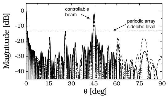
Figure 10: $101$-element modified-Fibonacci array with $d_{av}=0.874\lambda_{0}$ and $\eta=0$. Radiation pattern (array factor) $|{\hat{F}}(k_{0}\sin\theta)|$ in (10a) (with $|m|\leq 50$) for various values of scale ratio $\nu$, illustrating the controllable multibeam capability (see Sec. 5.2). —– $\nu=0.25$ ($S_{01}=-1.83$dB); - - - $\nu=0.5$ ($S_{01}=-6.37$dB); $\cdots\cdots$ $\nu=0.9$ ($S_{01}=-23.3$dB). Note that minor sidelobes never exceed the periodic-array sidelobe level (-13dB).

The direction $\beta_{01}$ can thus be steered, by varying $d_{av}/\lambda_{0}$, up to a maximum value $\beta_{01}^{(max)}=\arccos\left[\tau/(1+\tau)\right]\approx 51.83^{o}$, corresponding to the maximum spacing ($d_{av}=\lambda_{0}$) allowable to prevent emergence, in the visible range, of higher-order grating lobes. The amplitude $S_{01}$ can be controlled (from 0 to 1, in principle) by varying the scale ratio $\nu=d_{2}/d_{1}$ (from 1 to 0). One thus obtains a multibeam radiation pattern with the possibility of controlling the secondary beam amplitude. Results for the ($q_{1}=0,q_{2}=-1$) beam follow from symmetry considerations. Obvious fabrication-related issues prevent $\nu$ from being exceedingly small, but values of $\nu\approx 0.25$ are sufficient to achieve secondary beam amplitudes $\sim-2$dB. Figure 10 shows the radiation pattern (array factor) of a 101-element array, with $d_{av}/\lambda_{0}$ and $\nu$ chosen from (30) so as to create a secondary beam at $45^{o}$ with various amplitudes. It is observed that actual amplitude values are very close to the infinite-array predictions in (30), and that minor sidelobes never exceed the periodic-array sidelobe level (-13dB).

It is hoped that the above observations might open up new perspectives for reconfigurable arrays. Note that rational values of $\nu$ (commensurate scales) correspond to configurations interpretable as periodic arrays with aperiodically-distributed lacunas. In these cases, one can think of easily-implementable reconfigurable strategies, based on switching from single-beam (periodic array) to multibeam (modified-Fibonacci) radiation patterns, via on-off selection of a set of antenna elements, keeping the average inter-element spacing $d_{av}<\lambda_{0}$.

6 Conclusions and Perspectives

A simple illustrative example of wave interaction with quasiperiodic order has been discussed in connection with the radiation properties of 1-D antenna arrays, utilizing the modified-Fibonacci sequence. A “quasi-Floquet” analytic parameterization, based on a generalized Poisson summation formula, has been derived for infinite and semi-infinite arrays. Computational issues and potential applications have been briefly addressed.

It is hoped that the prototype study in this paper, through its instructive insights into some of the basic mechanisms governing wave interactions with quasiperiodic order, may lead to new applications in array radiation pattern control, in view of the additional degrees of freedom available in aperiodic structures. Accordingly, we are planning current and future investigations of modified-Fibonacci arrays that will emphasize the effects of the scale ratio parameter ($\nu=d_{2}/d_{1}$) on the input impedance as well as on the coupling to possible dielectric-substrate-induced leaky modes. Exploration of the radiation properties of antenna arrays based on other well-understood aperiodic sequences (e.g., Thue-Morse, period-doubling, Rudin-Shapiro [20]) is also being pursued.

Appendix
Pertaining to (10)–(13)

In [27], the modified-Fibonacci array spectrum in (10) is computed using two equivalent approaches, one directly based on the cut-and-project scheme described in Sec. 2.2 (see also Fig. 2), and the other based on an “average unit cell” method [32]. Although the two approaches are relatively simple in principle, their implementation is rather involved and not reported here for brevity. The reader is referred to [27], [32] for theoretical foundations and technical details, and to [40], [41] for an alternative approach applicable to rather general substitutional sequences. We point out that in [27], the result for the radiation spectrum is given in normalized form, with a non-explicit multiplicative constant, and assuming zero phasing ($\eta=0$). In the paper here, the possible presence of phasing is accounted for via the spectral shift $k_{0}\eta$ in (12). The calculation of the proper multiplicative constant in (10) (and hence that in (13)) has been accomplished by first observing that for the modified-Fibonacci sequence in (5), the number of array elements falling within a window of width $2\zeta$ approaches the ratio between the window width and the average inter-element spacing $d_{av}$ in (7), as $\zeta\rightarrow\infty$, i.e.,

$$\sum_{m=-\infty}^{\infty}\left[U\left(z_{m}+\zeta\right)-U\left(z_{m}-\zeta\right)\right]\sim\frac{2\zeta}{d_{av}},$$ (31)

with $U$ denoting the Heaviside step-function. It then follows from (1), assuming $\eta=0$ and recalling (31), that

$$\lim_{\zeta\rightarrow\infty}\frac{1}{2\zeta}\int_{-\zeta}^{\zeta}f(z)dz$$ (32)

$$= \lim_{\zeta\rightarrow\infty}\frac{1}{2\zeta}\sum_{m=-\infty}^{\infty}\left[U\left(z_{m}+\zeta\right)-U\left(z_{m}-\zeta\right)\right]$$

$$= \lim_{\zeta\rightarrow\infty}\frac{1}{2\zeta}\left(\frac{2\zeta}{d_{av}}\right)=\frac{1}{d_{av}}.$$

The proper multiplicative constants in (10) and (13) have accordingly been computed by requiring that (13) satisfy (32) for $\eta=0$.

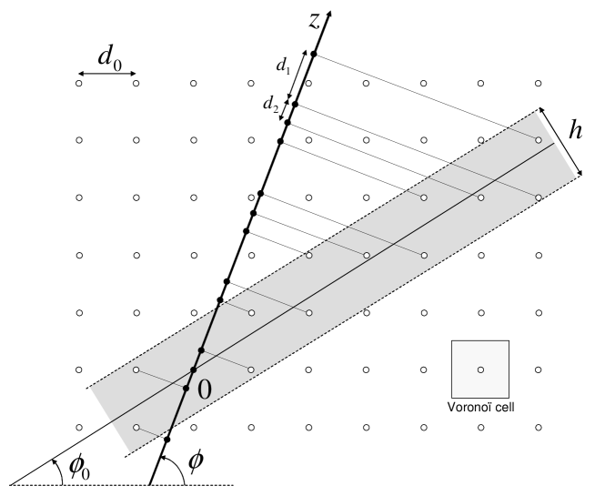
Figure 2: “Cut-and-project” graphic interpretation of the modified-Fibonacci sequence in (5). A 2-D square lattice of side $d_{0}=d_{1}\sqrt{1+\nu^{2}}$ is traversed by a straight line with slope $\tan\phi_{0}=1/\tau$, and those lattice points whose “Voronoï cell” (light-shaded square cell of side $d_{0}$ centered around the point) is crossed by the line (or, equivalently, those falling within the dark-shaded rectangular window of size $h=d_{0}(1+\tau)/\sqrt{2+\tau}$ centered around the line) are orthogonally projected onto another straight line ($z$-axis) with slope $\tan\phi=\nu$. For the standard-Fibonacci sequence ($\nu=1/\tau$), the two lines coincide ($\phi=\phi_{0}$).

References

- [1] D. Shechtman, I. Blech, D. Gratias, and J. W. Cahn, “Metallic phase with long-range orientational order and no translation symmetry,” Phys. Rev. Lett., vol. 53, No. 20, pp. 1951–1953, Nov. 1984.
- [2] D. Levine and P. J. Steinhardt, “Quasicrystals: A new class of ordered structures,” Phys. Rev. Lett., vol. 53, No. 26, pp. 2477–2480, Dec. 1984.
- [3] R. J. Mailloux, Phased Array Antenna Handbook. Boston (MA): Artech House, 1994.
- [4] B. D. Steinberg, “Comparison between the peak sidelobe of the random array and algorithmically designed aperiodic arrays,” IEEE Trans. Antennas Propagat., vol. 21, No. 3, pp. 366–370, May 1973.
- [5] Y.Kim and D. L. Jaggard, “The fractal random array,” Proc. of the IEEE, vol. 74, No. 9, pp. 1278–1280, Sept. 1986.
- [6] V. V. S. Prakash and R. Mittra, “An efficient technique for analyzing multiple frequency-selective-surface screens with dissimilar periods,” Microwave Opt. Technol. Letts., vol. 35, No. 1, pp. 23–27, Oct. 2002.
- [7] C. C. Chiau, X. Chen, and C. Parini, “Multiperiod EBG structure for wide stopband circuits,” IEE Proc. Microwaves, Antennas and Propagat., vol. 150, No. 6, pp. 489–492, Dec. 2003.
- [8] V. Pierro, V. Galdi, G. Castaldi, I. M. Pinto, and L. B. Felsen, “Radiation properties of planar antenna arrays based on certain categories of aperiodic tilings,” to be published in IEEE Trans. Antennas Propagat., vol. 53, No. 2, Feb. 2005.
- [9] B. Grünbaum and G. C. Shepard, Tilings and Patterns. New York (NY): Freeman, 1987.
- [10] M. Senechal, Quasicrystals and Geometry. Cambridge (UK): Cambridge University Press, 1995.
- [11] S. Vajda, Fibonacci and Lucas numbers, and the Golden Section: Theory and Applications. New York (NY): Halsted Press, 1989.
- [12] R. Merlin, K. Bajema, R. Clarke, F.-Y. Juang, and P. K. Bhattacharya, “Quasiperiodic GaAs-AlAs heterostructures,” Phys. Rev. Lett., vol. 55, 17, pp. 1768–1770, Oct. 1985.
- [13] R. Lifshitz, “Quasicrystals: A matter of definition,” Found. of Physics, vol. 33, No. 12, pp. 1703–1711, Dec. 2003.
- [14] M. Kohmoto, B. Sutherland, and K. Iguchi, “Localization of optics: Quasiperiodic media,” Phys. Rev. Lett., vol. 58, No. 23, pp. 2436 -2438, June 1987.
- [15] D. Würtz, T. Schneider, and M. P. Soerensen, “Electromagnetic wave propagation in quasiperiodically stratified media,” Physica A, vol. 148, No. 1-2, pp. 343–355, Feb. 1988.
- [16] A. Süto, “Singular continuous spectrum on a Cantor set of zero Lebesgue measure for the Fibonacci Hamiltonian,” J. Stat. Phys., vol. 56, pp. 525–531, 1989.
- [17] E. Diez, F. Domínguez-Adame, E. Maciá, and A. Sánchez, “Dynamical phenomena in Fibonacci semiconductor superlattices,” Phys. Rev. B, vol. 54, No. 23, pp. 16792–16798, Dec. 1996.
- [18] M. S. Vasconcelos, E. L. Albuquerque, and A. M. Mariz, “Optical localization in quasi-periodic multilayers,” J. Phys.: Condens. Matter, vol. 10, No. 26, pp. 5839–5849, July 1998.
- [19] E. Maciá, “Optical engineering with Fibonacci dielectric multilayers,” Appl. Phys. Lett., vol. 73, No. 23, pp. 3330–3332, Dec. 1998.
- [20] M. S. Vasconcelos and E. L. Albuquerque, “Transmission fingerprints in quasiperiodic multilayers,” Phys. Rev. B, vol. 59, No. 17, pp. 11128- 11131, May 1999.
- [21] Z. Ouyang, C. Jin, D. Zhang, B. Cheng, X. Meng, G. Yang, and J. Li, “Photonic bandgaps in two-dimensional short-range periodic structures,” J. Opt. A: Pure Appl. Opt., vol. 4, No. 1, pp. 23- 28, Jan. 2002.
- [22] E. Cojocaru, “Omnidirectional reflection from finite periodic and Fibonacci quasi-periodic multilayers of alternating isotropic and birefringent thin films,” Appl. Opt., vol. 41, No. 4, pp. 747–755, Feb. 2002
- [23] L. Dal Negro, C. J. Oton, Z. Gaburro, L. Pavesi, P. Johnson, A. Lagendijk, R. Righini, M. Colocci, and D. S. Wiersma, “Light transport through the band-edge states of Fibonacci quasicrystals,” Phys. Rev. Lett. vol. 90, 055501, Feb. 2003.
- [24] J. Baumberg, “When photonic crystals meet Fibonacci,” Phys. World, vol. 16, No. 4, p. 24, Apr. 2003.
- [25] J.-W. Dong, P. Han, and H.-Z. Wang, “Broad omnidirectional reflection band forming using the combination of Fibonacci quasi-periodic and periodic one-dimensional photonic crystals,” Chin. Phys. Lett., vol. 20, No. 11, pp. 1963–1965, Nov. 2003.
- [26] R. Ilan, E. Liberty, S. E.-D. Mandel, and R. Lifshitz, “Electrons and phonons on the square Fibonacci tiling,” Ferroelectrics, vol. 305, pp. 15–19, 2004.
- [27] P. Buczek, L. Sadun, and J. Wolny, “Periodic diffraction patterns for 1D quasicrystals,” preprint No. cond-mat/0309008 available at http://arxiv.org/abs/cond-mat/0309008.
- [28] H. Wei, C. Zhang, Y.-Y. Zhu, S.-N. Zhu, and N.-B. Ming, “Analytical expression for the Fourier spectrum of a quasi-periodic Fibonacci superlattice with components (),” Phys. Stat. Sol. (b), vol. 229, No. 3, pp. 1275–1282, Feb. 2002.
- [29] L. B. Felsen and F. Capolino, “Time-domain Green’s function for an infinite sequentially excited periodic line array of dipoles,” IEEE Trans. Antennas Propagat., vol. 48, No. 6, pp. 921–931, June 2000.
- [30] F. Capolino and L. B. Felsen, “Frequency- and time-domain Green’s function for a phased semi-infinite periodic line array of dipoles,” IEEE Trans. Antennas Propagat., vol. 50, No. 1, pp. 31–41, Jan. 2002.
- [31] M. Severin, “An analytical treatment of diffraction in quasiperiodic superlattices,” J. Phys.: Condens. Matter, vol. 1, No. 38, pp. 6771–6776, Sept. 1989.
- [32] J. Wolny, “Average unit cell approach to diffraction analysis of some aperiodic structures – decorated Fibonacci chain,” Czech. J. Phys., vol. 51, No. 4, pp. 409–419, Apr. 2001.
- [33] H. Bohr, Almost Periodic Functions. New York (NY): Chelsea, 1947.
- [34] A. S. Besicovitch, Almost Periodic Functions. New York (NY): Dover, 1954.
- [35] A. Papoulis, The Fourier Integral and Its Applications. New York (NY): McGraw-Hill, 1962.
- [36] L. Carin and L. B. Felsen, “Time-harmonic and transient scattering by finite periodic flat strip arrays: Hybrid (Ray)-(Floquet Mode)-(MOM) algorithm and its GTD interpretation,” IEEE Trans. Antennas Propagat., vol. 41, No. 4, pp. 412–421, Apr. 1993.
- [37] L. B. Felsen and L. Carin, “Diffraction theory and of frequency- and time-domain scattering by weakly aperiodic truncated thin-wire gratings,” J. Opt. Soc. Am. A, vol. 11, No. 4, pp. 1291–1306, Apr. 1994.
- [38] L. B. Felsen and E. Gago-Ribas, “Ray theory for scattering by two-dimensional quasiperiodic plane finite arrays,” IEEE Trans. Antennas Propagat., vol. 44 , No. 3, pp. 375–382, Mar. 1996.
- [39] A. Cucini, M. Albani, and S. Maci, “Truncated Floquet wave full-wave analysis of large phased arrays of open-ended waveguides with a nonuniform amplitude excitation,” IEEE Trans. Antennas Propagat., vol. 51, No. 6, pp. 1386–1394, June 2003.
- [40] M. Kolář, “New class of one-dimensional quasicrystals,” Phys. Rev. B, vol. 47, No. 9, pp. 5489–5492, Mar. 1993.
- [41] M. Kolář, B. Iochum, and L. Raymond, “Structure factor of 1D systems (superlattices) based on two-letter substitution rules: I. (Bragg) peaks,” J. Phys. A: Math. Gen., vol. 26, No. 24, pp. 7343–7366, Dec. 1993.