Efficient numerical integrators for stochastic models

Abstract

The efficient simulation of models defined in terms of stochastic differential equations (SDEs) depends critically on an efficient integration scheme. In this article, we investigate under which conditions the integration schemes for general SDEs can be derived using the Trotter expansion. It follows that, in the stochastic case, some care is required in splitting the stochastic generator. We test the Trotter integrators on an energy-conserving Brownian model and derive a new numerical scheme for dissipative particle dynamics. We find that the stochastic Trotter scheme provides a mathematically correct and easy-to-use method which should find wide applicability.

1 Introduction

The study of mesoscopic particle models such as Brownian dynamics (BD)[1], Dissipative Particle Dynamics (DPD) [2, 3], Smoothed Dissipative Particle Dynamics (SDPD) [4] and the Voronoi fluid particle model [5, 6] requires efficient integration methods that solve the appropriate stochastic equations of motion. In the past few years, several authors have considered improvements to the basic stochastic Euler schemes normally applied to these systems of equations, particularly in the context of “conventional” DPD. Groot & Warren [7], Pagonabarraga et al. [8] and Besold et al. [9] have reported various performance improvements to the basic schemes through the use of more sophisticated deterministic solvers, for example those that have been successfully employed for deterministic dynamical systems [10] including molecular dynamics (MD) simulations [11], such as the velocity and leapfrog Verlet algorithms. These traditional deterministic integrators provide significant improvements on the basic Euler solver albeit, being deterministic schemes, their behaviour is completely uncontrolled from a theoretical point of view and their order of convergence is not clear. In fact, these solvers arbitrarily leave out terms which should appear in a correct stochastic expansion. More recently, alternative schemes have been devised resulting from proper stochastic expansions [12, 13], and even from a Monte Carlo-based approach [14, 15] where the fluctuations are introduced via a thermostat (the deterministic dynamics is still dependent on the integrator).

A general method for deriving deterministic integrators is based on the Trotter expansion [1, 16]. For Hamiltonian systems, these schemes preserve the symplectic structure of the dynamics and conserve the dynamical invariants, ensuring that the long time behaviour is correctly captured. In fact, if a dynamical invariant $I$ exists then the discrete dynamics conserves exactly a virtual invariant $I^{\ast}$ which is bound to $I$ up to second order in $\Delta t$ [10]. An important feature of mesoscopic models is that they often recover a symplectic dynamics in some limit, an example being the DPD model for vanishing friction coefficient. It may be important to account for this quasi-symplectic property of the SDEs in the integration scheme by assuring that in the same limit the scheme is symplectic as well [17].

Recently, a first order stochastic generalisation of the Trotter expansion has been rigorously proved [18, 19]. In fact, for specific stochastic equations there exist schemes up to weak fourth order [20] or schemes corrected to reproduce more accurately the equilibrium distribution function [17]. The situation is less clear for a general SDE (such as Eq. (2) in Section 2), for which the application of the Trotter formula was overlooked in the literature, thereby generating some confusion in terms of how the Trotter formula can be used to split the stochastic equations. It is therefore useful to investigate the applicability of the Trotter formula in the most general case. This is of direct relevance for mesoscopic models which usually involve very large systems of SDEs.

The Trotter formula has been applied to devise efficient integrators for several specific mesoscopic models but often its use is limited to splitting the propagator into several terms which are then integrated using standard numerical schemes. This approach would correctly produce the order of accuracy expected for the dynamics but potentially would affect adversely the conservation of the dynamical invariants or even detailed balance. Examples include a numerical scheme suggested by a straightforward application of the Trotter rule to the Voronoi fluid particle model equations [21] which leads to time steps that are two orders of magnitude larger than the standard Euler scheme. In the context of the conventional DPD model, Shardlow [12, 13] presented a new scheme, which splits the stochastic and deterministic parts following the Trotter rule, and then integrates the fluctuation-dissipation generators using the Bruenger et al. scheme [22] tailored onto the DPD equations. For Brownian dynamics, Ricci & Ciccotti [23] derived a numerical integrator based on the Trotter expansion which integrates the propagators by using the Suzuki formula [24] to transform the time-ordered exponential solution of the Brownian dynamics equations into more tractable simple exponentials.

2 Stochastic Trotter schemes

Let us consider first a deterministic dynamical system $\mathbf{\dot{x}}(t)=\mathcal{L}[\mathbf{x}]$. The formal solution of this system is $\mathbf{x}(t)=\sum_{p=0}^{\infty}\frac{1}{p!}(\mathcal{L}t)^{p}[\mathbf{x}](\mathbf{x}_{0})(=e^{\mathcal{L}t}[\mathbf{x}](\mathbf{x}_{0}))$ as can be shown from the Taylor expansion around the initial condition $\mathbf{x}_{0}$. In general, the operator can be decomposed into simpler operators of the form $\mathcal{L}=\sum_{i}^{M}\mathcal{L}_{i}$. The Trotter formula (Strang [25]) provides a straightforward approximation to the time propagator

$$e^{\mathcal{L}t}=\left(\prod_{i=M}^{1}e^{\mathcal{L}_{i}\frac{\Delta t}{2}}\prod_{j=1}^{M}e^{\mathcal{L}_{j}\frac{\Delta t}{2}}\right)^{P}+O(\Delta t^{3})$$ (1)

where $t=\Delta tP$, $P$ is the number of time steps each of size $\Delta t$, and the ordering of the $i,j$ indices is important. In the case that two operators $\mathcal{A}$,$\mathcal{B}$ commute, i.e. $[\mathcal{A},\mathcal{B}]=\mathcal{AB}-\mathcal{BA}=0,$ then the approximate Trotter formula is indeed exact because the equations $e^{\mathcal{A}+\mathcal{B}}=e^{\mathcal{A}}e^{\mathcal{B}}=e^{\mathcal{B}}e^{\mathcal{A}}$ are valid. Because the Trotter formula decomposes the dynamics over the time interval $t$ into $P$ steps, it provides a discrete algorithm for the solution of the dynamics of the system. Well known examples of the deterministic Trotter expansion are velocity and position Verlet schemes for molecular dynamics simulations [1].

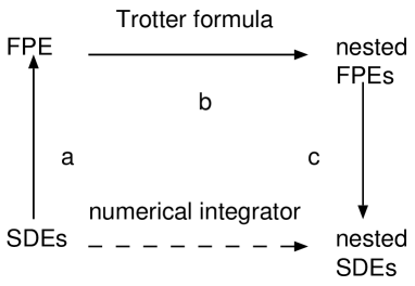
Figure 1: Diagram showing the derivation of SDE integrators by using the Trotter formula. Step (a) is the standard transformation from SDE to FPE formalism [26]. Step (b) decouples the FPE using the deterministic Trotter formula. Step (c) applies the reverse transformation from each decoupled FPE to the corresponding SDE in the order given in (b).

In the stochastic case, we define a $d$ dimensional stochastic process $\mathbf{x}_{t}=(x_{t}^{1},...,x_{t}^{d})$ with associated stochastic differential equation (SDE) in the Itô interpretation

$$dx_{t}^{k}=a^{k}(\mathbf{x}_{t})dt+\sum_{j=1}^{m}b^{kj}(\mathbf{x}_{t})dW_{t}^{j}$$ (2)

where $a^{k}(\mathbf{x}_{t})$ is the drift vector, $b^{kj}(\mathbf{x}_{t})$ is the diffusion matrix ($d$ variables, $m$ Wieners) and $dW_{t}^{j}$ the vector of independent increments of the $j$-th Wiener process. The mathematically equivalent Fokker-Planck equation (FPE) of Eq. (2) for the probability density $\rho(\mathbf{x},t)$ is

$${\partial_{t}}\rho=\mathcal{F}[\rho]$$ (3)

where $\mathcal{F}[\rho]=-\sum_{k}\frac{\partial}{\partial x^{k}}\left(a^{k}\rho\right)+\frac{1}{2}\sum_{k,l}\frac{\partial^{2}}{\partial x^{k}\partial x^{l}}\left(d^{kl}\rho\right)$ and $d^{kl}=\sum_{j}b^{kj}b^{lj}$ is the diffusion matrix.

Following the diagram depicted in Fig. (1), we translate the starting stochastic equation (2) into the corresponding Fokker-Planck equation (3) which has formal solution $\rho(\mathbf{x},t)=e^{\mathcal{F}t}[\rho](\rho_{0})$. The deterministic Trotter formula (1) can be applied to this formal solution by generally splitting the operator $\mathcal{F}=\sum_{i}\mathcal{F}_{i}$. Furthermore, if $\mathcal{F}_{i}$ is a Fokker-Planck operator itself, this picture of evolving the probability density using the Trotter formula has a counterpart at the level of the SDE which would allow us to devise a numerical integrator. However, not all decompositions $\mathcal{F}_{i}$ have Fokker-Planck form and therefore an associated SDE. We then proceed by progressively splitting the terms in the starting SDE, i.e the drift vector $a^{k}$ and the matrix $b^{kj}$, to verify Fokker-Planck form.

The drift terms do not present any special problem: that is any splitting of the vector

$$a^{k}=\sum_{\alpha}a^{k}_{\alpha},$$ (4)

produces Fokker-Plank drift-like terms which can be easily integrated as with any standard ordinary differential equation (ODE). The diffusion operator demands more care. The matrix $b^{kj}$ can be split into columns such as to give several systems of single noise equations, $b_{\alpha}^{kj}=b^{kj}\delta_{\alpha,j}$ which are different from zero only in the column corresponding to noise $\alpha=j$. By substituting $b^{kj}=\sum_{\alpha}b_{\alpha}^{kj}$ into the diffusive matrix $d^{kl}=\sum_{\alpha,\beta}\sum_{j}b_{\alpha}^{kj}b_{\beta}^{lj}$ we obtain

$$d^{kl}=\sum_{\alpha}\sum_{j}b_{\alpha}^{kj}b_{\alpha}^{lj}$$ (5)

which is split into several diffusive operators, because $\mathbf{b}_{\alpha}\cdot\mathbf{b}_{\beta}^{t}=0,\forall\alpha\neq\beta$, i.e. the correlations between different diffusive dynamics are zero. In this procedure, we decouple the diffusive dynamics in terms of the subdynamics corresponding to each independent Wiener process.

We are still left to integrate $m$ single noise SDEs. We can try to decompose further each system of single noise SDEs into separate scalar SDEs. For each noise $j$, we set $b_{\alpha}^{kj}={b}^{kj}\delta_{\alpha,k}$ such that substituting in $d^{kl}$ we have

$$d^{kl}=\sum_{\alpha,\beta}\sum_{j}b_{\alpha}^{kj}b_{\beta}^{lj},$$ (6)

which cannot be reduced to Fokker-Planck form for all terms. This means that we cannot split variables over terms of the same noise to derive the integrator. In fact, in order to apply the diagram of Fig. (1) and in particular step (c), we need to have all the terms in Fokker-Planck form to derive the corresponding SDEs. In principle, one could also try to separate the diffusion matrix $d^{kl}$ itself into several simpler matrices $d^{kl}=\sum_{\alpha}d_{\alpha}^{kl}$ provided that each matrix $d_{\alpha}^{kl}$ is positive definite, but then the non-unique square-roots of the matrices $d_{\alpha}^{kl}$ have to be computed in order to recover the SDEs. Practically, this is very difficult in general.

Finally, we must be able to compute the solution of the SDE corresponding to the $i$ term $\mathcal{F}_{i}$ in order to write down the integration scheme. This is possible for simple SDEs, otherwise we can take advantage of the splitting between the drift and diffusion generators. The analytical solution of SDEs with zero drift is conveniently calculated in the Stratonovich interpretation for the stochastic integral (for a reference on Stratonovich integrals see [26]). In fact, the standard rules of ordinary calculus apply and the SDEs are effectively integrated like ordinary differential equations by formally considering $dW$ as $dt$. An Itô SDE like Eq. (2) is transformed into the equivalent Stratonovich form with the usual rules for the drift

$$\underline{a}^{k}=a^{k}-\frac{1}{2}\sum_{j=1}^{m}\underline{L}^{j}b^{kj}$$ (7)

where $\underline{L}^{j}=\sum_{h=1}^{d}b^{h,j}\frac{\partial}{\partial x^{h}}$ and the noise term is interpreted accordingly as $dx_{t}^{k}=\underline{a}^{k}(\mathbf{x}_{t})dt+\sum_{j=1}^{m}b^{kj}(\mathbf{x}_{t})\circ dW_{t}^{j}$ (see [26]).

As the Trotter formula approximates the dynamics (3) of the probability distribution $\rho$ up to second order in time, we expect that at the SDE level the accuracy of the method is weak second-order [26], i.e. moments are accurate to second order. Effectively, the proposed decomposition at the FPE level allows us to reduce the time-ordered exponential solution of SDE (2) in terms of simple exponentials up to second order provided that the generators for the same noise are not split.

3 An energy-conserving Brownian model

The oldest model for a stochastic system is the Langevin equation for a Brownian particle. In the one dimensional case, the SDE governing the velocity of the particle is $dv=-vdt+(2T)^{1/2}dW$ where we have selected units in which the mass of the particle and friction coefficient are unity and $T$ is the dimensionless bath temperature. This equation predicts an exponential decay of the velocity and, consequently, of the kinetic energy of the Brownian particle which goes into the fluid surrounding the particle. For illustrative purposes, we can construct an energy-conserving model in which we include the energy $\epsilon$ of the fluid system, a Lagrangian reference system and a conservative force. We use the dimensionless equations in Stratonovich form

$$dr =vdt$$

$$dv =F(r)dt-vdt+(2\alpha\epsilon)^{1/2}\circ dW_{t},$$

$$d\epsilon =v^{2}dt-(2\alpha\epsilon)^{1/2}v\circ dW_{t},$$ (8)

where $F=-\frac{\partial V(r)}{\partial r}$ is the conservative force and $\alpha$ is a dimensionless heat capacity of the fluid. The above SDEs have as a dynamical invariant the total energy $E=E_{0}=V(r)+\frac{v^{2}}{2}+\epsilon$. Generalisations of the SDEs (8) to higher dimensions and multiple particles are indeed fundamental building-blocks of several mesoscopic models.

In practice, it is not necessary to move to a Fokker-Planck description to derive the integration scheme. The derivation in section (2) shows that we can simply apply the Trotter formula (1) over the generators of the SDEs (8) provided that we do not split the stochastic generator for the same noise. The SDEs (8) is written in the form $d{\bf x}_{t}=\mathcal{L}[{\bf x}]dt+\mathcal{S}[{\bf x}]\circ d{\bf W}_{t}$, where ${\bf x}=(r,v,\epsilon)$ and the deterministic and stochastic generators are respectively $\mathcal{L}=\mathcal{L}_{1}+\mathcal{L}_{2}+\mathcal{L}_{3}+\mathcal{L}_{4}$ and $\mathcal{S}=\mathcal{S}_{1}+\mathcal{S}_{2}$,

$$\mathcal{L}_{1} = v\partial/\partial r;~{}~{}\mathcal{L}_{2}=F\partial/\partial v;~{}~{}\mathcal{L}_{3}=-v\partial/\partial v;~{}~{}\mathcal{L}_{4}=v^{2}\partial/\partial\epsilon;$$

$$\mathcal{S}_{1} = (2\alpha\epsilon)^{1/2}\partial/\partial v;~{}~{}\mathcal{S}_{2}=-(2\alpha\epsilon)^{1/2}v\partial/\partial\epsilon.$$ (9)

The generators $\mathcal{S}_{1}$ and $\mathcal{S}_{2}$ cannot be split and integrated independently using the Trotter formula because they refer to the same noise. However, the solution for $\mathcal{S}$ can be directly computed by applying standard calculus on the system of two equations $d{\bf x}_{t}=\mathcal{S}[{\bf x}]\circ d{\bf W}_{t}$; the solution is given by

$$e^{\mathcal{S}\Delta W_{\Delta t}}[{\bf x}]:\begin{array}[l]{l}\epsilon\rightarrow C\cos\left(\sqrt{\alpha}\Delta W_{\Delta t}+\arccos(\sqrt{\epsilon/C})\right)^{2},\\ v\rightarrow sign(v)\sqrt{2C}\sin\left(\sqrt{\alpha}\Delta W_{\Delta t}+\arccos(\sqrt{\epsilon/C})\right),\end{array}$$ (10)

where $sign(x)=1$ if $x\geq 0$ and $sign(x)=-1$ if $x<0$. Both variables are updated starting from the same initial values and $C=\epsilon+v^{2}/2$ is computed before the update. The deterministic generators are easily integrated

$$e^{\mathcal{L}_{1}\Delta t}[{\bf x}] : r\rightarrow r+v\Delta t;~{}~{}e^{\mathcal{L}_{2}\Delta t}[{\bf x}]:v\rightarrow v+F\Delta t,$$

$$e^{\mathcal{L}_{3}\Delta t}[{\bf x}] : v\rightarrow v\exp(-\Delta t);~{}~{}e^{\mathcal{L}_{4}\Delta t}[{\bf x}]:\epsilon\rightarrow\epsilon+v^{2}\Delta t.$$ (11)

The solutions of these differential equations can be nested following any given order to obtain different integration schemes. A possible numerical scheme is

$$e^{\mathcal{S}\Delta W_{\Delta t/2}}e^{\mathcal{L}_{4}\frac{\Delta t}{2}}e^{\mathcal{L}_{3}\frac{\Delta t}{2}}e^{\mathcal{L}_{2}\frac{\Delta t}{2}}e^{\mathcal{L}_{1}\Delta t}e^{\mathcal{L}_{2}\frac{\Delta t}{2}}e^{\mathcal{L}_{3}\frac{\Delta t}{2}}e^{\mathcal{L}_{4}\frac{\Delta t}{2}}e^{\mathcal{S}\Delta W^{\prime}_{\Delta t/2}},$$ (12)

where $\Delta W^{\prime}_{\Delta t/2}$ and $\Delta W_{\Delta t/2}$ are two random numbers drawn from a zero mean normal distribution with standard deviation $\sqrt{\Delta t/2}$. We note that the stochastic propagator of this scheme conserves energy exactly (for any time step size), therefore the conservation of energy depends only on the approximation introduced in the deterministic part.

As already stated, it is not possible to decompose the stochastic generator $\mathcal{S}$ into two independent stochastic scalar equations using the Trotter formula. Unfortunately, this approach is what would follow if one was to apply naively the Trotter formula to SDE (8). The resulting scheme would not be second order and would conserve energy poorly. For instance, this is the case for the scheme

$$e^{\mathcal{S}_{1}\Delta W_{\Delta t/2}}e^{\mathcal{S}_{2}\Delta W_{\Delta t/2}}e^{\mathcal{L}_{4}\frac{\Delta t}{2}}e^{\mathcal{L}_{3}\frac{\Delta t}{2}}e^{\mathcal{L}_{2}\frac{\Delta t}{2}}e^{\mathcal{L}_{1}\Delta t}e^{\mathcal{L}_{2}\frac{\Delta t}{2}}e^{\mathcal{L}_{3}\frac{\Delta t}{2}}e^{\mathcal{L}_{4}\frac{\Delta t}{2}}e^{\mathcal{S}_{2}\Delta W^{\prime}_{\Delta t/2}}e^{\mathcal{S}_{1}\Delta W^{\prime}_{\Delta t/2}},$$ (13)

where the stochastic propagators are

$$e^{\mathcal{S}_{1}\Delta W_{\Delta t}}[{\bf x}] : v\rightarrow v+\sqrt{2\alpha\epsilon}\Delta W_{\Delta t},$$

$$e^{\mathcal{S}_{2}\Delta W_{\Delta t}}[{\bf x}] : \epsilon\rightarrow(\sqrt{\epsilon}-\sqrt{2\alpha}v/2\Delta W_{\Delta t})^{2}.$$ (14)

Interesting, there is a possibility to apply a Trotter-like rule to devise second order weak integrators even for the decomposition $\mathcal{S}=\mathcal{S}_{1}+\mathcal{S}_{2}$. To do this the noises have to be advanced by $\frac{\Delta W_{\Delta t}}{2}=(weak)\Delta W_{\Delta t/4}$, where by $=(weak)$ we mean that moments of both sides are equal to second order. Note that for the Trotter expansion it should be $\Delta W_{\Delta t/2}=W_{t+\Delta t/2}-W_{t}$. The scheme is written as

$$e^{\mathcal{S}_{1}\Delta W_{\Delta t/4}}e^{\mathcal{S}_{2}\Delta W_{\Delta t/4}}e^{\mathcal{L}_{4}\frac{\Delta t}{2}}e^{\mathcal{L}_{3}\frac{\Delta t}{2}}e^{\mathcal{L}_{2}\frac{\Delta t}{2}}e^{\mathcal{L}_{1}\Delta t}e^{\mathcal{L}_{2}\frac{\Delta t}{2}}e^{\mathcal{L}_{3}\frac{\Delta t}{2}}e^{\mathcal{L}_{4}\frac{\Delta t}{2}}e^{\mathcal{S}_{2}\Delta W_{\Delta t/4}}e^{\mathcal{S}_{1}\Delta W_{\Delta t/4}},$$ (15)

where we use the same realization of the noise $\Delta W_{\Delta t/4}$. The second order weak convergence can be verified by a direct comparison with a second order stochastic expansion and intuitively understood by formally considering $\Delta W$ as $\Delta t$. We stress that the resulting scheme does not correspond to a stochastic Trotter expansion, but rather to a second order approximation of the propagator. This method provides a way to write an integration scheme even in cases where it is impractical to compute the solution of the generator $\mathcal{S}$ altogether. However, wherever possible, this approach should be avoided or limited to the smallest generator because the resulting integration scheme may loose important structural features of the dynamics (as in the example of SDEs (8)).

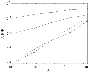
Figure 2: Average of the maximum relative error of the energy for the SDE (8) over 10 independent runs up to $t=1$ for the Trotter schemes (12) circles, (15) squares and the incorrect Trotter scheme (13) triangles. The deterministic Trotter scheme for Eq. (8) with $\alpha=0,v_{0}=1,\epsilon_{0}=1/2$ is plotted with dotted lines for reference.

We validated numerically the integration schemes (12) and (15) as well as the incorrect one (13). The simulations were run using the bistable potential $V(r)=\beta(r^{4}-2r^{2})$ with $\alpha=1$, $\beta=1$ and initial conditions $r_{0}=0,~{}v_{0}=0$ and $\epsilon_{0}=1$. The average relative error for the total energy $\Delta E/E$ for different time step lengths $\Delta t$ is shown in Fig. 2. The error is computed by averaging the maximum error reached by $t=1$ over 10 independent runs. The stochastic-Trotter scheme (12) conserves the energy with the same accuracy as the deterministic Trotter scheme (computed using $\alpha=0$). The scheme (15) is consistent with first order accuracy (it is second order for single time step error), while the incorrect scheme (13) does not conserve energy with first order accuracy. Note that the order for the cumulative error is one less than the single time step error. Clearly, the energy conservation performance of the Trotter scheme (12) is a direct consequence of the exact integration of its stochastic component which is impossible to achieve by other general schemes.

4 A Trotter integration scheme for dissipative particle dynamics

We now apply the stochastic Trotter expansion to the equations of dissipative particle dynamics. The DPD model consists of a set of $N$ particles moving in continuous space. Each particle $k$ is defined by its position $\mathbf{r}_{k}$ and its momentum $\mathbf{p}_{k}$ and mass $m$. The dynamics is specified by a set of Langevin equations very similar to the molecular dynamics equations, but where in addition to the conservative forces there are dissipative and fluctuating forces as well

$$d\mathbf{{r}}_{k} = \mathbf{p}_{k}/mdt,$$

$$d\mathbf{{p}}_{k} = \sum_{l\neq k}^{N}\mathbf{e}_{kl}\left[a_{kl}F_{c}(r_{kl})dt-\gamma/m\omega_{D}(r_{kl})(\mathbf{e}_{kl}\cdot\mathbf{p}_{kl})dt+\sigma\omega_{R}(r_{kl})dW^{t}_{kl}\right],$$ (16)

where $F_{c}(r)$ is the conservative pair interaction force weighted by positive and symmetric parameters $a_{kl}$, $\mathbf{r}_{kl}={\bf r}_{k}-{\bf r}_{l}$ is the distance between the particle $k$ and particle $l$, ${r}_{kl}$ its length and ${\bf e}_{kl}={\bf r}_{kl}/r_{kl}$. The weight functions $\omega_{D},\omega_{R}$ usually have finite range $r_{c}$ and are related by $\omega_{D}(r_{kl})=\omega_{R}^{2}(r_{kl})$ in order to satisfy detailed balance. This condition ensures that the equilibrium state is Gibbsian and sets the value of its temperature to $T_{0}=\frac{\sigma^{2}}{2\gamma k_{B}}$. A typical selection is $\omega_{R}(r_{kl})=\omega(r_{kl})$ with

$$\omega(r)=\left\{\begin{array}[]{cc}1-\frac{r}{r_{c}}&r<r_{c}\\ 0&r\geq r_{c}.\end{array}\right.$$ (17)

The conservative force ${F}_{c}(r_{kl})=-\frac{\partial V(r_{kl})}{\partial r_{k}}$ is usually chosen to be of the form ${F}_{c}(r_{kl})=w(r_{kl})$.

The generator of DPD equations (16) is $\mathcal{L}=\sum_{k}\mathcal{L}^{k}_{r}+\sum_{k,l\neq k}\left(\mathcal{D}^{kl}+\mathcal{S}^{kl}\right),$ where

$$\mathcal{L}^{k}_{r} = \mathbf{p}_{k}/m\partial/\partial{\bf r}_{k};~{}~{}\mathcal{S}^{kl}=\sigma\omega_{R}(r_{kl})\mathbf{e}_{kl}\partial/\partial{\bf p}_{k};$$

$$\mathcal{D}^{kl} = a_{kl}F_{c}(r_{kl})\mathbf{e}_{kl}\partial/\partial{\bf p}_{k}-\gamma/m\omega_{D}(r_{kl})(\mathbf{e}_{kl}\cdot\mathbf{p}_{kl})\mathbf{e}_{kl}\partial/\partial{\bf p}_{k}.$$ (18)

In the DPD model the momentum is conserved because the forces between interacting particles $k$ and $l$ satisfy Newton’s third law. We split the DPD equations in order to satisfy this requirement. The conservative and fluctuation-dissipation generators for the pair interaction $k$, $l$ give

$$d{\bf x}=(\mathcal{D}^{kl}+\mathcal{D}^{lk})[{\bf x}]dt+(\mathcal{S}^{kl}+\mathcal{S}^{lk})[{\bf x}]dW^{t}_{kl}$$ (19)

where ${\bf x}=({\bf r}_{1},{...},{\bf r}_{N},{\bf p}_{1},{...},{\bf p}_{N})$. The solution is computed by noting that $d\mathbf{{p}}_{k}+d\mathbf{{p}}_{l}=0$ and $d\mathbf{{p}}_{k}=\frac{1}{2}d\mathbf{{p}}_{kl}$ where $d\mathbf{{p}}_{kl}=d\mathbf{{p}}_{k}-d\mathbf{{p}}_{l}$. The equation for $d\mathbf{{p}}_{kl}$ can be solved for the component of the radial direction because from the form of the SDEs (16) it follows that $d\mathbf{{p}}_{kl}=d(\mathbf{{p}}_{kl}\cdot\mathbf{e}_{kl})\mathbf{e}_{kl}$. Let us call $p^{e}_{kl}=\mathbf{{p}}_{kl}\cdot\mathbf{e}_{kl}$; then we have an Ornstein-Uhlenbeck process

$$dp^{e}_{kl}=Adt-Bp^{e}_{kl}dt+CdW^{t}_{kl},$$ (20)

where $A=2a_{kl}F_{c}(r_{kl})$, $B=2\gamma/m\omega_{D}$ and $C=2\sigma\omega_{R}$, which has analytical solution [26]

$$p^{e}_{kl}(t)=e^{-B\Delta t}p^{e}_{kl}(t_{0})+A\int_{t_{0}}^{t}e^{B(s-t)}ds+C\int_{t_{0}}^{t}e^{B(s-t)}dW_{s},$$ (21)

where $\Delta t=t-t_{0}$, $t_{0}$ being the initial time. The solution (21) of the Ornstein-Uhlenbeck process requires the generation of coloured noise based on a numerical scheme itself [27]. In fact, the stochastic process $p^{e}_{kl}(t)$ has stationary correlation function for $t,s\rightarrow\infty$ with finite $|t-s|$ given by

$$<p^{e}_{kl}(t)p^{e}_{kl}(s)>=\frac{A^{2}}{B^{2}}+\frac{C^{2}}{2B}\exp(-B|t-s|).$$ (22)

A version of the method to generate coloured noise [27] adapted to Eq. (21) results in the scheme

$$\Delta{p}^{e}_{kl}=\left(\mathbf{{p}}_{kl}\cdot{\bf e}_{kl}-\frac{a_{kl}F_{c}}{\frac{\gamma}{m}w_{D}}\right)\left(e^{-2\frac{\gamma}{m}\omega_{D}\Delta t}-1\right)+\frac{\sigma\omega_{R}\sqrt{1-e^{-4\gamma/m\omega_{D}\Delta t}}}{\sqrt{\gamma/m\omega_{D}}}\xi^{kl},$$ (23)

where $\xi^{kl}=\xi^{lk}$ are normal distributed with zero mean and variance one ($N(0,1)$) and $\Delta{p}^{e}_{kl}={p}^{e}_{kl}(t)-{p}^{e}_{kl}(t_{0})$ .

The propagator $\mathcal{K}^{kl}$ for $\mathbf{p}_{k}$ and $\mathbf{p}_{l}$ is then given by

$$\mathcal{K}^{kl}_{\Delta t}[{\bf x}]:(\mathbf{{p}}_{k},\mathbf{{p}}_{l})\rightarrow\left(\mathbf{{p}}_{k}+\frac{1}{2}\Delta{p}^{e}_{kl}{\bf e}_{kl},~{}~{}\mathbf{{p}}_{l}-\frac{1}{2}\Delta{p}^{e}_{kl}{\bf e}_{kl}\right).$$ (24)

The remaining position update is given by

$$e^{\mathcal{L}^{k}_{r}\Delta t}[{\bf x}]:{\bf r}_{k}\rightarrow{\bf r}_{k}+{\bf p}_{k}/m\Delta t.$$ (25)

We note that $\mathcal{L}^{k}_{r}$ commutes with $\mathcal{L}^{l}_{r}$, therefore we can use the exact formula $e^{\sum_{k}\mathcal{L}^{k}_{r}\Delta t}=\prod_{k=1}^{N}e^{\mathcal{L}^{k}_{r}\Delta t}$.

The DPD scheme is finally given by the following Trotter integrator

$${\bf x}(t+\Delta t)\rightarrow\prod_{k=1,l=1}^{N}\mathcal{K}^{kl}_{\Delta t/2}~{}~{}\prod_{k=1}^{N}e^{\mathcal{L}^{k}_{r}\Delta t}\prod_{k=N,l=N}^{1}\mathcal{K}^{kl}_{\Delta t/2}~{}{\bf x}(t).$$ (26)

In practice the integration algorithm consists of the following steps: for the interaction pairs k,l update the momentum half timestep according to the propagator (24), where $\xi^{kl}=\xi^{lk}$ are drawn from a normal distribution with zero mean and variance one; iterate over particles $k$ updating the position according to (25); finally, update pairs k,l in reverse order again using the propagator (24) but with new noise $\xi^{\prime}_{kl}$. This algorithm requires the calculation of the pair-list only once per iteration and has the same complexity as a simple DPD velocity-Verlet scheme (DPD-VV [7]).

We test this integration scheme using the open-source code mydpd [28] written in simple C++ and implementing the DPD models described here with periodic boundary conditions. The simulations are run with $N=4000$ particles, $a_{kl}=25$, $\gamma=4.5$, $\sigma=3$, $m=1$, $r_{c}=1$ in a three dimensional periodic box $(L,L,L)$ with $L=10$. These settings give a particle density $\rho=4$ and equilibrium temperature $k_{B}T=1$. In our implementation, the computational cost of each scheme averaged over several iterations indicates that the Trotter scheme is 60% more costly than the simple DPD-VV but 10% faster than the Shardlow S1 scheme (which costs almost twice than DPD-VV). The equilibrium temperature for the DPD-Trotter scheme of Eq. (26), DPD-VV [7] and Shardlow [12] schemes is reported in Table 1. The DPD-Trotter scheme recovers the equilibrium temperature better than DPD-VV, and as accurately as Shardlow’s scheme. This difference depends on the implicit scheme used by Shardlow for the integration of the pair interaction. In our case, we have used an exact integration Eq. (21) which, however, requires the generation of coloured noise [27] which is by itself a numerical scheme. Considering the accuracy of the equilibrium temperature and the computational cost, both DPD-Trotter and Shardlow schemes are integrators of comparable performance for the DPD equations. A more detailed study of the equilibrium properties of the fluid is necessary to assess the accuracy in reproducing the equilibrium distribution and other statistical properties.

Table 1: Equilibrium temperature for the DPD-Trotter, Shardlow and DPD-VV schemes for different time steps. The average of the kinetic temperature $<k_{B}T>$ is computed over a simulation of duration $t=1000$. The standard deviation of the estimates, computed by block-averaging, is less than $\pm 5\times 10^{-4}$.

$\Delta t$	DPD-Trotter (scheme Eq. (26))	Shardlow [12]	DPD-VV [7]
0.05	1.0136	1.0138	1.0411
0.02	1.0020	1.0018	1.0097
0.01	1.0007	1.0005	1.0043

5 Conclusions

The stochastic Trotter schemes can provide efficient integrators for stochastic models with dynamical invariants by fully taking into account the underlying stochastic character. The stochastic Trotter formula can be applied to any model based on SDEs and should find wide applicability provided that some care is used to decouple the stochastic dynamics for the same noise. These types of stochastic schemes offer the flexibility to easily tailor the integrator to the specific model, thereby integrating exactly important parts of the dynamics. This stochastic Trotter scheme is a second order weak scheme, but, more important, in our examples it provides very good conservation of the dynamical invariants.

Acknowledgements

We thank G. Tessitore for useful comments. This work was partially supported by the SIMU Project, European Science Foundation. GDF is supported by the EPSRC Integrative Biology project GR/S72023. M.S. and P.E. thank the Ministerio de Ciencia y Tecnología, Project BFM2001-0290.

References

- [1] M. P. Allen and D. J. Tildesley, Computer Simulations of Liquids, Oxford University Press, Oxford, 1987.
- [2] P. J. Hoogergrugge and J. M. V. A. Koelman, Europhys. Lett. 19 (1992) 155.
- [3] P. Español, P. Warren, Europhys. Lett. 30 (1995) 191.
- [4] P. Español, M. Revenga, Phys. Rev. E 67 (2003) 026705.
- [5] E. G. Flekkøy, P. V. Coveney, G. De Fabritiis, Phys. Rev. E 62 (2000) 2140.
- [6] M. Serrano, P. Español, Phys. Rev. E 64 (2001) 046115.
- [7] R. D. Groot, P. B. Warren, J. Chem. Phys. 107 (1997) 4423.
- [8] I. Pagonabarraga, M. H. J. Hagen, D. Frenkel, Europhys. Lett. 42 (1998) 377.
- [9] G. Besold, I. Vattualainen, M. Karttunen, J. M. Polson, Phys. Rev. E 62 (2000) R7611.
- [10] P. J. Channell, C. Scovel, Nonlinearity 3 (1990) 231.
- [11] M. Tuckerman, B. J. Berne, J. Chem. Phys. 97 (1992) 1990.
- [12] T. Shardlow, SIAM J. Sci. Comput. 24 (2003) 1267.
- [13] P. Nikunen, M. Karttunen, I. Vattulainen, Comp. Phys. Comm. 153 (2003) 407.
- [14] C. P. Lowe, Europhys. Lett. 47 (1999) 145.
- [15] E. A. J. F. Peters, Europhys. Lett. 66 (2004) 311.
- [16] H. F. Trotter, Proc. Amer. Math. Soc. 10 (1959) 545–551.
- [17] R. Mannella, Phys. Rev. E 69 (2004) 041107.
- [18] G. Tessitore, J. Zabczyk, Semigroup Forum 63 (2001) 115.
- [19] F. Kuhnemund, Bi-continuous semigroup on spaces with two-topologies: theory and applications, Ph.D. thesis, Eberhard Karls Universität Tübingen, Germany (2001).
- [20] H. A. Forbert, S. A. Chin, Phys. Rev. E 63 (2000) 016703.
- [21] G. De Fabritiis, P. V. Coveney, Comp. Phys. Comm. 153 (2003) 209.
- [22] A. Bruenger, C. L. Brooks III, M. Karplus, Chem. Phys. Lett. 105 (1984) 495.
- [23] A. Ricci, G. Ciccotti, Mol. Phys. 101 (2003) 1927.
- [24] M. Suzuki, Proc. Jpn. Acad. B 69 (1993) 161.
- [25] G. Strang, SIAM J. Numer. Anal. 5 (1968) 506.
- [26] P. E. Kloeden, E. Platen, Numerical solution of stochastic differential equations, Springer-Verlag, Berlin, 1992.
- [27] R. F. Fox, I. R. Gatland, R. Roy, G. Vemuri, Phys. Rev. A 38 (1988) 5938.
- [28] Available online at http://www.openmd.org/mydpd.