Bremsstrahlung from dense plasmas and the Landau-Pomeranchuk-Migdal effect

Abstract

The suppression of the bremsstrahlung cross section due to multiple scattering of the emitting electrons is an important effect in dense media (Landau-Pomeranchuk-Migdal effect). Here, we study the emission from a dense, fully-ionized and non-relativistic hydrogen plasma. Using the dielectric approach, we relate optical properties such as emission and absorption to equilibrium force-force correlation functions, which allow for a systematic perturbative treatment with the help of thermodynamic Green functions. By considering self-energy and vertex corrections, medium modifications such as multiple scattering of the emitting electrons are taken into account. Results are presented for the absorption coefficient as a function of the frequency at various densities. It is shown that the modification of the inverse bremsstrahlung due to medium effects becomes more significant in the low frequency and high density region.
Keywords: bremsstrahlung, laser-induced plasmas, dynamical collision frequency, LPM effect

I 1. INTRODUCTION

In a fully ionized plasma, bremsstrahlung and inverse bremsstrahlung are the only emission and absorption processes, respectively. For partially ionized plasmas these processes contribute to some extent to the continuous emission/absorption spectrum. We introduce the emission coefficient $j(\omega)$ as the rate of radiated energy per unit volume, frequency and solid angle, and the absorption coefficient $\alpha(\omega)$ as the relative attenuation of the intensity of electromagnetic waves propagating in the medium per unit length. For a thermally equilibrated plasma, these quantities are linked by Kirchhoff’s law griem

$$j(\omega)=L(\omega)\alpha(\omega)\;\;\;,$$ (1)

with the Planck distribution $L(\omega)=\hbar\omega^{3}/\left[4\pi^{3}c^{2}(\exp(\hbar\omega/k_{\mathrm{B}}T)-1)\right]$. Thus, it is sufficient to study one or the other, i.e. $j(\omega)$ or $\alpha(\omega)$ . Here, we choose the absorption coefficient $\alpha(\omega)$.

The absorption spectrum can be determined according to Quantum Electrodynamics (QED) itzykson from the interaction part of the QED Lagrangian

$${\mathcal{L}}_{\rm int}(x)=\sum_{c}Z_{c}ej^{c}_{\mu}(x)A^{\mu}(x),$$ (2)

$x$ being a four-dimensional space-time variable. This Lagrangian describes a minimal coupling between the particle current $j_{\mu}^{c}$ and the vector potential $A^{\mu}$. The index $c$ denotes the species of the particles involved, carrying the charge $Z_{c}e$. Introducing a Hamiltonian $H$, the transition rate between asymptotically free states of electrons $|\,\boldsymbol{p}_{\mathrm{in}}\,\rangle,|\,\boldsymbol{p}_{\mathrm{out}}\,\rangle$ with the energies $E^{\mathrm{e}}_{\mathrm{in}},E^{\mathrm{e}}_{\mathrm{out}}$ respectively, follows from Fermi’s Golden rule as

$$w_{\rm in,out}=\frac{2\pi}{\hbar}\Big{|}\langle\boldsymbol{p}_{\rm out}|H_{\mathrm{int}}|\boldsymbol{p}_{\rm in}\rangle\Big{|}^{2}\delta(E_{\rm in}^{\rm e}+\hbar\omega-E_{\rm out}^{\rm e})~{},$$ (3)

with $H_{\mathrm{int}}=-\int\mathrm{d}^{3}x\,\mathcal{L}_{\mathrm{int}}(x)$. Assuming single, uncorrelated scattering from different ions only, the absorption coefficient is given by

$$\alpha(\omega)=n_{\rm i}\Omega_{0}\int\frac{\Omega_{0}\mathrm{d}^{3}p_{\rm in}}{(2\pi)^{3}}\,\frac{\Omega_{0}\mathrm{d}^{3}p_{\rm out}}{(2\pi)^{3}}\;f(E^{\mathrm{e}}_{\rm in})\frac{1}{c}w_{\rm in,out}~{}.$$ (4)

Here, $n_{\rm i}\Omega_{0}$ is the total number of ions in the volume $\Omega_{0}$ and $w_{\rm in,out}$ is the transition probability that a photon of momentum $\boldsymbol{k}=\boldsymbol{p}_{\rm out}-\boldsymbol{p}_{\rm in}$ and polarization $\lambda$ is absorbed by a single electron of momentum $\boldsymbol{p}_{\rm in}$ in the Coulomb potential of an ion, leaving the process with momentum $\boldsymbol{p}_{\rm out}$. The momentum distribution function of the incoming electrons is denoted as $f(E^{\mathrm{e}}_{\rm in})=\left[\exp\left((\hbar^{2}p^{2}_{\rm in}/2m_{\mathrm{e}}-\mu_{\mathrm{e}})/k_{\mathrm{B}}T\right)+1)\right]^{-1}$. The factor $1/c$ arises due to the current of incoming photons.

Evaluating the transition rate in Born approximation

$$\langle\boldsymbol{p}_{\rm out}|H_{\mathrm{int}}|\boldsymbol{p}_{\rm in}\rangle = \frac{Z_{i}e^{2}\hbar^{2}}{\epsilon_{0}m_{\rm e}\Omega_{0}}\sqrt{\frac{e^{2}}{2\hbar\epsilon_{0}\Omega_{0}\hbar\omega}}\,\frac{\left(\boldsymbol{p}_{\rm out}-\boldsymbol{p}_{\rm in}\right)_{z}}{|{\boldsymbol{p}}_{\rm out}-{\boldsymbol{p}}_{\rm in}|^{2}}$$ (5)

results in the well known Bethe-Heitler cross section beth:proc.roy.soc36 ; Heitler .

In the low frequency limit, the Bethe-Heitler cross section behaves roughly like $1/\omega$. Within QED, this infrared-divergence is discussed as a consequence of the neglect of vertex corrections holstein . The infrared-divergent terms can be shown to cancel with corresponding contributions to the form factor of the source particle which is a manifestation of the Ward-Takahashi identities bjor:qfield .

In the non-relativistic limit and for soft photons, the absorption coefficient for a hydrogen plasma ($Z_{\mathrm{i}}=1$) is given by

$$\alpha^{\rm B}(\omega) = \frac{C}{\hbar\omega^{3}}\,n_{\rm e}\,n_{\rm i}\,\sinh\left(\frac{\hbar\omega}{2k_{\rm B}T}\right)\,K_{0}\left(\frac{\hbar\omega}{2k_{\rm B}T}\right)~{},$$ (6)

where $C^{-1}=3\sqrt{2}\epsilon_{0}^{3}\pi^{3/2}m_{\rm e}^{3/2}c\left(k_{\rm B}T\right)^{1/2}/e^{6}$ and $K_{0}(x)=\int_{0}^{\infty}\cos(x\sinh t)\mathrm{d}t$ is the modified Bessel function. Here, the electron density $n_{\mathrm{e}}$ has been introduced, which is equal to the ion density $n_{\mathrm{e}}=n_{\mathrm{i}}$ in charge neutral systems.

This Born approximation can be improved by taking Coulomb wave functions for the initial and final states. In this case, an analytic result for the absorption coefficient was given by Sommerfeld S . Due to the occurrence of hyper-geometric functions, simpler approximations such as the Born-Elwert approximation E have been developed. In the classical limit, the Sommerfeld expression reduces to a result obtained by Kramers earlier K .

In a dense plasma, the influence of the collective behavior of the system and the modification of single-particle properties of the emitting and absorbing particles as well as the bremsstrahlung photons are important. Retaining the single-scattering picture of Eq. (4), medium effects can be taken into account e.g. by a modification of the potential. Instead of a Coulomb potential, a static or dynamically screened potential should be used B1 . A quantum-statistical approach based on a systematic perturbative treatment of the force-force correlation function has been developed in Ref. rein:pre00 , for an application to inverse bremsstrahlung see Ref. wier:phpl01 .

How does multiple scattering of the emitting electron change the cross section? This question was first treated by Landau and Pomeranchuk land:dokl53 in a semi-classical way and soon afterwards by Migdal migd:physrev56 using quantum statistical methods. They showed that the account of successive collisions leads to a suppression of the bremsstrahlung cross section compared to the Bethe-Heitler result at photon energies low against the energy of the scattering electron. Both Bethe-Heitler and Landau-Pomeranchuk-Migdal (LPM) theory give the same result in the limiting cases of high photon energies and/or low densities, i.e., in those cases where the Born approximation is applicable. Migdal’s result has been rederived more recently using different methods, e.g., path-integral calculations zakh96 ; zakh98 and quantum kinetic equations kosh:jphysa02 . A comprehensive overview of theoretical approaches is given in klei:revmodphys99 . There, it is also pointed out that the LPM effect might play an important rôle for the emission/absorption spectrum of a plasma even in the non-relativistic regime due to the large number of free charge carriers. Other aspects of the emission of radiation are also under consideration such as a coherent state description of photon emission wang:jphys01 ; czac:phle03 .

Due to the large energies required to observe notable effects, it took quite a long time until experiments could unambiguously approve LPM theory. Experimental investigations have been performed since the late 1950’s using high energy electrons (some MeV to GeV) from cosmic rays fowl:phil.mag59 ; varf:jetp60 ; lohr:pr61 ; kasa:prd85 ; stra91 and accelerators varf:jetp75 . These early experiments suffered from poor statistics and were unable to confirm LPM theory. More recent experiments at SLAC anto:prd97 and CERN bak:nucl88 ; hans:prl03 ; hans:prd04 have indeed shown the LPM effect.

Migdal’s theory is not completely microscopic but relies on the definition of a macroscopic parameter, namely the coherence length $l$, initially introduced by Ter-Mikaelyan klei:revmodphys99 and first applied to the theory of bremsstrahlung by Landau and Pomeranchuk land:dokl53 . The coherence length gives the scale of photon energy, below which the suppression of bremsstrahlung becomes important. It is basically determined by the density of the medium. Knoll and Voskresensky knol:annals96 were the first to treat the question of the LPM effect in the context of a many particle system, where every constituent has to be regarded as an emitter of bremsstrahlung. They were able to show a suppression of the emission/absorption spectrum at low frequencies by using medium modified single particle propagators. The particles are assigned a finite lifetime $\tau$, given by the width of their spectral function $\Gamma=\hbar/\tau$. However, this quantity is not calculated from a microscopic approach, but simply set as a parameter. It is related to the aforementioned coherence length by the simple relation $\tau\simeq l/c$ voskr_pc03 .

In this work, we present a completely microscopic calculation of the absorption spectrum, where the spectral function of the electron is obtained in a self consistent manner. Thus, we present for the first time a fully microscopic treatment of the LPM effect for a many-particle system. The absorption coefficient is defined in linear response theory and is expressed through thermodynamical correlation functions using a diagram technique equivalent to the well known Feynman diagrams krae . Medium effects are accounted for systematically in terms of self-energy and vertex corrections. We show that the Bethe-Heitler bremsstrahlung spectrum follows from this approach in lowest order perturbation theory using free particle propagators. The account of coherent successive scattering, as in LPM theory, can be achieved by a partial summation of self-energy diagrams. This procedure leads to a finite width of the single-particle spectral function which reflects the modification of the energy-momentum dispersion relation due to the medium. It is found that the absorption coefficient calculated on the basis of these medium modified propagators is significantly altered in the low frequency range in comparison to the Born approximation. In the high frequency limit as well as in the low density limit, the Born approximation is reproduced. Thus, the main features of LPM theory can be rederived within our microscopic approach.

II 2. LINEAR RESPONSE THEORY

We consider the interaction of soft photons with a non-relativistic, homogeneous plasma. A key quantity to describe the propagation of electro-magnetic waves in a medium is the dielectric tensor $\epsilon_{ij}({\boldsymbol{k}},\omega)$ jack . In the isotropic case, the tensor can be decomposed into a transverse $\epsilon_{\rm t}(k,\omega)$ and a longitudinal $\epsilon_{\mathrm{l}}(k,\omega)$ part with respect to the wave vector $\boldsymbol{k}$. Here and in the following, we take $\boldsymbol{k}$ to point along the $z$-axis, $\boldsymbol{k}=k\boldsymbol{e}_{z}$. In the long-wavelength limit $\boldsymbol{k}\to 0$, the longitudinal and the transverse part coincide $\epsilon(\omega)=\lim_{k\to 0}\epsilon_{\mathrm{l}}(k,\omega)=\lim_{k\to 0}\epsilon_{\mathrm{t}}(k,\omega)$. The absorption coefficient can be obtained from the dielectric function according to

$$\alpha(\omega) = \frac{\omega}{c}\frac{{\rm Im}\,\epsilon(\omega)}{n(\omega)}\;\;\;,$$ (7)

where the index of refraction $n(\omega)$ is also linked to the dielectric function by

$$n(\omega) = \frac{1}{\sqrt{2}}\left({\rm Re}\,\epsilon(\omega)+\left|\epsilon(\omega)\right|\right)^{1/2}\;\;\;.$$ (8)

The relation between $\epsilon_{\mathrm{l}}(k,\omega)$ and the longitudinal response function $\chi_{\mathrm{l}}(k,\omega)$

$$\epsilon_{\mathrm{l}}(k,\omega)=\frac{1}{1-\frac{e^{2}}{\epsilon_{0}k^{2}}\chi_{\mathrm{l}}(k,\omega)}~{},$$ (9)

allows for a microscopic approach to the dielectric function. Within linear response theory, the Kubo formula relates the response function to the current-current correlation function maha

$$\chi_{\rm l}({\boldsymbol{k}},\omega) = i\beta\Omega_{0}\frac{k^{2}}{\omega}\,\langle J_{k}^{z};J_{k}^{z}\rangle_{\omega+i\eta}\;\;\;,$$ (10)

where the correlation functions for two observables $A,B$ are defined according to

$$(A;B) = {1\over\beta}\int\limits_{0}^{\beta}\mathrm{d}\tau\,{\rm Tr}[A(-i\hbar\tau)B^{\dagger}\rho_{0}]\;\;\;,$$

$$\langle A;B\rangle_{\omega+i\eta} = \int\limits_{0}^{\infty}\mathrm{d}t\,\mathrm{e}^{i(\omega+i\eta)t}\,(A(t);B)~{}.$$ (11)

The time dependency of the operators is taken in the Heisenberg picture. The current density operator is given as

$${\boldsymbol{J}}_{k}={1\over\Omega_{0}}\sum_{c,\boldsymbol{p}}{e_{c}\over m_{c}}\hbar\boldsymbol{p}\,a^{\dagger}_{c,\boldsymbol{p}-\boldsymbol{k}/2}a_{c,\boldsymbol{p}+\boldsymbol{k}/2}\;\;\;.$$ (12)

$a^{\dagger}_{c,p}$ and $a_{c,p}$ are creation and annihilation operators for momentum states, respectively. $c$ labels the species and further quantum numbers such as spin, $\Omega_{0}$ is a normalization volume, $\rho_{0}$ is the equilibrium statistical operator, $\beta=1/(k_{\rm B}T)$ is the inverse temperature. Note, that in Eq.(10), a small but finite imaginary part $\eta$ has been added. In the final results, the limit $\eta\to 0$ is taken.
The inverse response function can also be expressed as rein:pre00

$$\chi^{-1}_{\rm l}(\boldsymbol{k},\omega)={i\over\beta\Omega_{0}}{\omega\over k^{2}}{1\over(J^{z}_{k};J^{z}_{k})^{2}}\left[-i\omega(J^{z}_{k};J^{z}_{k})+\langle\dot{J}^{z}_{k};\dot{J}^{z}_{k}\rangle_{\omega+i\eta}-{\langle\dot{J}^{z}_{k};J^{z}_{k}\rangle_{\omega+i\eta}\langle J^{z}_{k};\dot{J}^{z}_{k}\rangle_{\omega+i\eta}\over\langle J^{z}_{k};J^{z}_{k}\rangle_{\omega+i\eta}}\right]\;\;\;.$$ (13)

This transformation of the current-current correlation function into a force-force correlation function $\langle\dot{J}^{z}_{k};\dot{J}^{z}_{k}\rangle_{\omega+i\eta}$ with

$$\boldsymbol{\dot{J}}=\frac{i}{\hbar}\left[H,\boldsymbol{J}\right]~{},$$ (14)

which has the meaning of a force as the time derivative of momentum, is more suited for a perturbative treatment rein:pre00 . Also, it is convenient to introduce a generalized collision frequency $\nu(\omega)$ in analogy to the Drude relation rein:pre00

$$\epsilon(\omega) = 1\,-\,\frac{\omega_{\rm pl}^{2}}{\omega\,\left(\omega+i\nu\left(\omega\right)\right)}\;\;\;,$$ (15)

where $\omega_{\rm pl}^{2}=\sum_{c}\,n_{c}e_{c}^{2}/(\epsilon_{0}m_{c})$ is the squared plasma frequency.
By comparison with Eq. (9), we establish an expression for the collision frequency in terms of correlation functions

$$\nu(\omega)=\frac{\beta\Omega_{0}}{\epsilon_{0}\omega_{\rm pl}^{2}}\,\lim_{k\to 0}\,\left[\big{\langle}\,\,\dot{\!\!J}_{k}^{z},\,\,\dot{\!\!J}_{k}^{z}\big{\rangle}_{\omega+i\eta}\,-\,\frac{\langle\dot{J}^{z}_{k};J^{z}_{k}\rangle_{\omega+i\eta}\,\langle J^{z}_{k};\dot{J}^{z}_{k}\rangle_{\omega+i\eta}}{\langle J^{z}_{k};J^{z}_{k}\rangle_{\omega+i\eta}}\right]\;\;\;,$$ (16)

taking into account that $(J^{z}_{k};J^{z}_{k})=\epsilon_{0}\omega_{\rm pl}^{2}/\beta\Omega_{0}$ is an exactly known quantity. Further details can be found in Ref. rein:pre00 . Making use of Eq. (7), the absorption coefficient can be expressed as

$$\alpha(\omega)=\frac{\omega_{\rm pl}^{2}}{c}\frac{{\rm Re}\;\nu(\omega)}{(\omega^{2}-2\omega\,{\rm Im}\,\nu(\omega)+|\nu(\omega)|^{2})n(\omega)}\;\;\;.$$ (17)

In the high frequency limit $\omega\gg\omega_{\rm pl}$, the index of refraction is unity and the collision frequency is small compared to the frequency $\omega$. Then, we can consider the approximation

$$\alpha(\omega) = \frac{\omega_{\rm pl}^{2}}{c\,\omega^{2}}\,\mbox{Re}\,\nu(\omega)\;=\;\frac{\beta\Omega_{0}}{c\epsilon_{0}\omega^{2}}\,{\rm Re}\,\big{\langle}\,\,\dot{\!\!J}_{0}^{z},\,\,\dot{\!\!J}_{0}^{z}\big{\rangle}_{\omega+i\eta}\;\;\;,$$ (18)

where the collision frequency is given in the form of a force-force correlation function, cf. Ref. rein:pre00 . Thus, the absorption coefficient is directly proportional to the real part of the force-force correlation function, which itself can be determined using perturbation theory.

As well known, the deviation of the diffraction index $n(\omega)$ from unity at frequencies near the plasma frequency $\omega_{\mathrm{pl}}$ is responsible for the so-called dielectric suppression of the bremsstrahlung spectrum. We refer to the pioneering work of Ter-Mikaelyan ter . In our approach, making use of Eqs. (8), (15), and (16), the index of refraction can be determined from the force-force correlation function. However, due to the choice of the frequency range in consideration ($\omega\gg\omega_{\mathrm{pl}}$), this effect will not be considered in the present work. We will focus only on the medium effects obtained directly from the evaluation of the force-force correlation function.

III 3. GREEN FUNCTION APPROACH AND DENSITY EFFECTS

A convenient starting point for a perturbative treatment of the force-force correlation function is the representation in terms of a Green function $G_{\dot{J}\dot{J}}$ in the limit $k\to 0$ zuba2

$$\langle\dot{J}_{0}^{z},\dot{J}_{0}^{z}\rangle_{\omega+i\eta} = \frac{i}{\beta}\int_{-\infty}^{\infty}\!\frac{\mathrm{d}\bar{\omega}}{\pi}\,\frac{1}{\omega+i\eta-\bar{\omega}}\,\frac{1}{\bar{\omega}}\,{\rm Im}\,G_{\dot{J}\dot{J}}(\bar{\omega}+i\eta)~{}.$$ (19)

By exploiting Dirac’s identity

$$\lim_{\eta\to 0}\frac{1}{x\pm i\eta} = {\cal P}\frac{1}{x}\mp i\pi\delta(x)~{},$$ (20)

the real part of the force-force correlation function is evaluated to

$${\rm Re}\,\langle\dot{J}_{0}^{z},\dot{J}_{0}^{z}\rangle_{\omega+i\eta}=\frac{1}{\beta\omega}{\rm Im}\,G_{\dot{J}\dot{J}}(\omega+i\eta)~{}.$$ (21)

Thus, the absorption coefficient reads in the high-frequency limit

$$\alpha(\omega) = \frac{\pi\Omega_{0}}{c\epsilon_{0}\omega^{3}}\,{\rm Im}\,G_{\dot{J}\dot{J}}(\omega+i\eta)~{}.$$ (22)

The time derivative of the electron current density operator is calculated as

$$\dot{J}^{z}_{0,{\rm e}}=\frac{i}{\hbar}\big{[}H,J^{z}_{0,{\rm e}}\big{]}=\frac{ie}{m_{\mathrm{e}}\Omega_{0}}\,\sum_{\boldsymbol{pkq}}v_{q}^{\rm ei}q_{z}a^{\dagger}_{\mathrm{e},\boldsymbol{p}}\,a^{\dagger}_{\mathrm{i},\boldsymbol{k}}\,a_{\mathrm{i},\boldsymbol{k}-\boldsymbol{q}}\,a_{\mathrm{e},\boldsymbol{p}+\boldsymbol{q}}$$ (23)

with the Hamiltonian

$$H = \sum_{c,\boldsymbol{k}}E^{c}_{k}a^{\dagger}_{c,\boldsymbol{k}}a_{c,\boldsymbol{k}}+\frac{1}{2}\sum_{c,d\atop\boldsymbol{kpq}}v^{cd}_{q}a^{\dagger}_{c,\boldsymbol{k}+\boldsymbol{q}}a^{\dagger}_{d,\boldsymbol{p}-\boldsymbol{q}}a_{d,\boldsymbol{p}}a_{c,\boldsymbol{k}}~{}$$ (24)

and $E_{k}^{c}=\hbar^{2}k^{2}/2m_{c}$. The spin is not given explicitly but is included into the free-particle quantum number $c$. Due to conservation of total momentum of electrons, only electron-ion collisions contribute to Eq.(23). With Eq.(23), we identify the Green function as a four particle Green function. Its diagrammatic representation is shown in FIG. 1, l.h.s. Here, $G_{4}$ denotes a four-particle Green function that contains all interactions between the considered particles wier:phpl01 . We perform a sequence of approximations by selecting certain diagrams contributing to $G_{4}$. Considering the electron-ion interaction determining the force $\dot{J}^{z}_{0,{\rm e}}$ only in lowest order, i.e. in Born approximation, but the full correlations within the electron and ion subsystem, respectively, we are led to the middle of FIG. 1 (b) showing only those diagrams which can be factorized into two polarization bubbles. $\Pi_{\mathrm{e}}$ denotes the electronic polarization function, $\Pi_{\mathrm{i}}$ is the corresponding ionic quantity. In this way, we keep the description of the single scattering event on the level of the Born approximation. However, higher order interactions between the full electron and ion subsystem such as a ladder approximation (t-matrix) are ignored, cf. also Ref. rein:pre00 . The t-matrix corrections and in particular the reproduction of the Sommerfeld result S have been studied in Ref. wier:phpl01 .

III.1 A. Born approximation

As a simple example and prerequisite for further improvements, we consider the Born approximation. In this case, $G_{4}$ is a product of four single particle propagators and all single particle propagators are replaced by free propagators. We obtain for the Green function the diagram given in FIG. 1, r.h.s. Details of the calculation are discussed in App. A. For a Maxwellian plasma ($f(E^{\mathrm{e}}_{p})=n_{\mathrm{e}}\Lambda_{\mathrm{e}}^{3}/2\,\exp(-\beta E^{\mathrm{e}}_{p})$), we obtain

$${\rm Im}\,G^{\mathrm{Born}}_{\dot{J}\dot{J}}(\omega) = \frac{n_{\rm i}n_{\rm e}\Lambda_{e}^{3}e^{6}(1-e^{-\beta\hbar\omega})}{24\pi^{3}\epsilon_{0}^{2}\hbar^{4}\omega^{2}}\int\!\mathrm{d}E^{\mathrm{e}}_{p}\,e^{-\beta E^{\mathrm{e}}_{p}}\times$$ (25)

$$\times\left(-2\frac{\sqrt{E^{\mathrm{e}}_{p}}\ \sqrt{\hbar\omega+E^{\mathrm{e}}_{p}}\,\hbar^{2}\kappa^{2}/m_{\mathrm{e}}}{(\hbar\omega+\hbar^{2}\kappa^{2}/2m_{\mathrm{e}})^{2}+2E^{\mathrm{e}}_{p}\,\hbar^{2}\kappa^{2}/m_{\mathrm{e}}}+\frac{1}{2}\ln\left|\frac{\left(\sqrt{E^{\mathrm{e}}_{p}+\hbar\omega}+\sqrt{E^{\mathrm{e}}_{p}}\right)^{2}+\hbar^{2}\kappa^{2}/2m_{\mathrm{e}}}{\left(\sqrt{E^{\mathrm{e}}_{p}+\hbar\omega}-\sqrt{E^{\mathrm{e}}_{p}}\right)^{2}+\hbar^{2}\kappa^{2}/2m_{\mathrm{e}}}\right|\right).$$

Note, that the spin-degeneracy factor $1/2$ for fermions is compensated by a factor $2$ from the summation over spin variables in the calculation of the correlation functions. $\Lambda_{\mathrm{e}}=(2\pi\hbar^{2}/m_{\mathrm{e}}k_{\mathrm{B}}T)^{1/2}$ is the thermal de-Broglie wavelength. $\kappa$ occurs due to the use of a statically screened potential of Debye-Hückel type

$$v_{q}^{\rm ei}=-\frac{Z_{\rm i}e^{2}}{\epsilon_{0}\Omega_{0}(q^{2}+\kappa^{2})}~{},$$ (26)

with $\kappa^{2}=\sum_{c}n_{c}Z^{2}_{c}e^{2}/(\epsilon_{0}k_{\mathrm{B}}T)$, to ensure convergence at $\omega=0$. For $\omega\neq 0$, we can consider the Coulomb limit $\kappa=0$. Performing the integration with the help of

$$\int\limits_{0}^{\infty}{\mathrm{d}x\over x}\mathrm{e}^{-(a/x-bx)^{2}}={\rm e}^{2ab}K_{0}(2ab)\;\;\;,$$ (27)

we arrive at Eq. (6). Note, that this result is sometimes also written as Hutch

$$\alpha^{\rm Born}(\omega)={n_{\rm i}n_{\rm e}\Lambda_{\mathrm{e}}^{3}e^{6}\over 24\hbar^{4}\omega^{3}\epsilon_{0}^{3}c\pi^{3}}(1-\mathrm{e}^{-\beta\hbar\omega})\int\limits_{0}^{\infty}\mathrm{d}E^{\mathrm{e}}_{p}\,\mathrm{e}^{-\beta E^{\mathrm{e}}_{p}}\ln\left({\sqrt{E^{\mathrm{e}}_{p}+\hbar\omega}+\sqrt{E^{\mathrm{e}}_{p}}\over\sqrt{E^{\mathrm{e}}_{p}+\hbar\omega}-\sqrt{E^{\mathrm{e}}_{p}}}\right)~{}.$$ (28)

It is instructive to study the different terms in Eq.(28) in more detail: The integrand contains the distribution function (Maxwell distribution). Furthermore, a logarithm that depends on both electron and photon energy appears. Taken with appropriate prefactors, this logarithm is equal to the differential cross section for inverse bremsstrahlung in the non-relativistic limit (Bethe-Heitler formula) jack . Thus, we have a quite reasonable relation between the absorption coefficient as a macroscopic property and the underlying microscopic process, namely inverse bremsstrahlung. The absorption spectrum is obtained through integration of the cross section of the microscopic process weighted with the distribution function of the absorbing particles.
The absorption coefficient in Born approximation suffers the same logarithmic divergence in the limit $\omega\to 0$ (infrared divergence) as the non-relativistic limit of the Bethe-Heitler formula.
We will now show how the Born approximation can be improved. As already mentioned above, improvements based on a more sophisticated description of the single scattering process via a t-matrix approach have been obtained recently wier:phpl01 . Effects due to dynamical screening have also been considered. Both effects remove the infrared divergence mentioned before. In this work, we want to include medium effects such as the successive scattering of the absorbing particles on ions during the absorption of the photon, a process becoming more important with increasing density. This is also the basic idea of the LPM effect.

The correction in lowest order to Born which takes account of medium effects in the propagator can be achieved by performing either one self-energy insertion or one vertex correction in the sense of Ward-Takahashi identities. In diagrammatic terms, this means

(29)

We use $i^{+}$ to indicate loops with ionic propagators. The first loop on the r.h.s. yields the Born result as shown previously, in the following we have the self-energy and the vertex correction, respectively.
However, one does not obtain a finite result from this ansatz in the case of the self-energy correction. Instead, a partial summation of all self-energy terms leading to a spectral function is necessary. The results are presented in subsection 3.C. In constrast, the last diagram of Eq. (29) describing the vertex correction gives a finite contribution as shown in subsection 3.D. A full self-consistent treatment of the vertex, i.e. solving the corresponding Bethe-Salpeter equation krae , has not yet been performed.

III.2 B. Spectral function

We now discuss the influence of multiple scattering of the source particles (electrons) on ions. This can be accounted for by using dressed propagators in the calculation of the force-force correlation function, i.e. by replacing the free electron Green function by the expression

$$G_{\mathrm{e}}(\boldsymbol{p},z_{\nu})=\int\limits_{-\infty}^{\infty}\frac{\mathrm{d}\hbar\omega}{2\pi}\frac{A_{\rm e}(\boldsymbol{p},\hbar\omega)}{z_{\nu}-\hbar\omega}~{},$$ (30)

where $A_{\mathrm{e}}(\boldsymbol{p},\hbar\omega)$ is the electronic spectral function. According to Dyson’s equation krae , the Green function can be represented by a complex electron self-energy $\Sigma_{\mathrm{e}}(\boldsymbol{p},z_{\nu})$,

$$G_{\mathrm{e}}(\boldsymbol{p},z_{\nu}) =$$

$$= \frac{1}{z_{\nu}-E^{\mathrm{e}}_{p}-\Sigma_{\mathrm{e}}(\boldsymbol{p},z_{\nu})}~{}.$$

We perform the analytic continuation of the discrete Matsubara frequencies into the upper half of the complex energy plane via $z_{\nu}\to\hbar\omega+i\eta$ and decompose the self-energy into the real and imaginary part, $\Sigma_{\mathrm{e}}(\boldsymbol{p},\hbar\omega+i\eta)=\Delta_{\mathrm{e}}(\boldsymbol{p},\hbar\omega)-i\Gamma_{\mathrm{e}}(\boldsymbol{p},\hbar\omega)/2$. Then, the spectral function is related to the self-energy:

$$A_{\mathrm{e}}(\boldsymbol{p},\hbar\omega)=\frac{\Gamma_{\mathrm{e}}(\boldsymbol{p},\hbar\omega)}{(\hbar\omega-E^{\mathrm{e}}_{p}-\Delta_{\mathrm{e}}(\boldsymbol{p},\hbar\omega))^{2}+\Gamma^{2}_{\mathrm{e}}(\boldsymbol{p},\hbar\omega)/4}~{}.$$ (31)

For the self-energy, we describe the scattering of the electron on an ion by a statically screened ion potential, cf. Eq.(26).
The Hartree term vanishes due to charge neutrality. The Fock term of the electron self-energy is not relevant, since we assume a non degenerate system. The self-consistent first loop correction to the Hartree-Fock self-energy due to the electron-ion interaction is given by the diagram

$$\Sigma_{\mathrm{e}}(\boldsymbol{p},z_{\nu})\ =\ \parbox{56.37271pt}{ \includegraphics[width=56.37271pt,clip]{eq_sel.eps}}~{}.$$ (32)

This approximation can be improved by taking into account a partial summation of further loops, leading to the GW approximation for the self-energy maha .
After analytic continuation of the Matsubara Green function we have

$$\Sigma_{\rm e}(\boldsymbol{p},\hbar\omega+i\eta)=n_{\rm i}\int{\mathrm{d}^{3}q\over(2\pi)^{3}}\left|v_{q}^{\rm ei}\right|^{2}{1\over\hbar\omega+i\eta-E_{\boldsymbol{p+q}}^{\rm e}-\Sigma_{\rm e}(\boldsymbol{p+q},\hbar\omega+i\eta)}~{}.$$ (33)

Eq. (33) can be solved numerically by iteration starting from a suitable initialization.

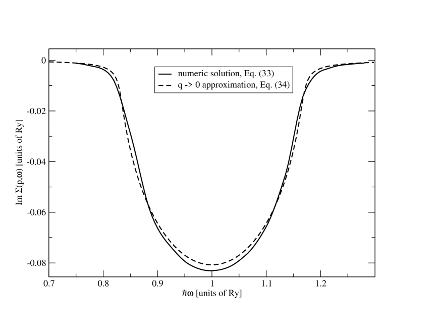
Figure 2: Solution of Eq. (33) for the imaginary part of the self-energy. Both, the full solution and the approximation with $q=0$ coincide to a large extent. The wave vector $p$ is taken as $p=1\,a_{B}^{-1}$. The parameters are $n_{\mathrm{e}}=10^{-6}\,a_{\mathrm{B}}^{-3}$ and $k_{\mathrm{B}}T=2\ \mathrm{Ry}=27.2\ \mathrm{eV}$.

From the form of the screened potential Eq. (26), we note that the main contribution to the integral in Eq. (33) arises from terms with small momentum $q$. Therefore, we will discuss an approximation where the argument $\boldsymbol{p}+\boldsymbol{q}$ in the self-energy is replaced by $\boldsymbol{p}$, i.e. $\Sigma_{\mathrm{e}}(\boldsymbol{p}+\boldsymbol{q},\hbar\omega)\approx\Sigma_{\mathrm{e}}(\boldsymbol{p},\hbar\omega)$ on the r.h.s. This ansatz is justified as can be seen in FIG. 2, where we show the full solution of Eq. (33) and the approximative solution for the set of parameters $n_{\mathrm{e}}=10^{-6}\,a_{\mathrm{B}}^{-3}$ and $k_{\mathrm{B}}T=2\ \mathrm{Ry}=27.2\ \mathrm{eV}$. After dropping the shift of the momentum variable in the self-energy, the $q$ integral can be performed analytically. The result

$$\Sigma_{\mathrm{e}}(\boldsymbol{p},\hbar\omega+i\eta)=-\frac{n_{\mathrm{i}}m_{\mathrm{e}}e^{4}}{4\pi\epsilon_{0}^{2}\hbar^{2}}\frac{1}{\kappa}\Bigg{[}\kappa^{2}+p^{2}-2\frac{m_{\mathrm{e}}}{\hbar^{2}}(\hbar\omega+i\eta-\Sigma_{\mathrm{e}}(\boldsymbol{p},\hbar\omega+i\eta))-2i\kappa\sqrt{2\frac{m_{\mathrm{e}}}{\hbar^{2}}(\hbar\omega+i\eta-\Sigma_{\mathrm{e}}(\boldsymbol{p},\hbar\omega+i\eta))}\Bigg{]}^{-1}\;,$$

(34)

is solved numerically for the real and imaginary part. In FIG. 3 l.h.s. (a), we show the self-energy, the dispersion relation, and the resulting spectral function obtained from a self-consistent solution of Eq. (34). The spectral function in FIG. 3 shows a broadened quasi-particle resonance at the energy $\hbar\omega=\hbar^{2}(p^{2}+\kappa^{2})/2m_{\mathrm{e}}$. As expected, its shape is primarily determined by the imaginary part of the self-energy. This can be seen by a comparison of $A_{e}(p,\omega)$ with $\Gamma_{e}(p,\omega)$.

We mention, that analytic constraints on the self-energy function such as Kramers-Kronig relations

$${\rm Im}\,\Sigma_{\mathrm{e}}(\boldsymbol{p},\hbar\omega)=\int\limits_{-\infty}^{\infty}\frac{\mathrm{d}\omega^{\prime}}{\pi}\frac{{\rm Re}\,\Sigma_{\mathrm{e}}(\boldsymbol{p},\hbar\omega^{\prime})}{\omega^{\prime}-\omega}~{},\quad{\rm Re}\,\Sigma_{\mathrm{e}}(\boldsymbol{p},\hbar\omega)=\int\limits_{-\infty}^{\infty}\frac{\mathrm{d}\omega^{\prime}}{\pi}\frac{{\rm Im}\,\Sigma_{\mathrm{e}}(\boldsymbol{p},\hbar\omega^{\prime}+i\eta)}{\omega^{\prime}-\omega}\;\;\;,$$ (35)

as well as the first sum-rule for the spectral function

$$\int\limits_{-\infty}^{\infty}\frac{\mathrm{d}\hbar\omega}{2\pi}A_{\mathrm{e}}(\boldsymbol{p},\hbar\omega)=1\;\;\;,$$ (36)

are fulfilled within the numerically achievable precision.

For the sake of comparison, we discuss a simplified calculation in which we neglect the self-consistent propagator and replace it by a free propagator. Thus, the self-energy on the r.h.s. of Eq. (32) disappears. Then we find

$$\Sigma^{0}_{e}(\boldsymbol{p},\hbar\omega+i\eta) = -\frac{n_{\mathrm{i}}me^{4}}{4\pi\epsilon_{0}^{2}\hbar^{2}}\frac{1}{\kappa}\Bigg{[}\kappa^{2}+p^{2}-2\frac{m_{\mathrm{e}}}{\hbar^{2}}(\hbar\omega+i\eta)-2i\kappa\sqrt{2\frac{m_{\mathrm{e}}}{\hbar^{2}}(\hbar\omega+i\eta)}\Bigg{]}^{-1}~{},$$ (37)

which can be separated into real and imaginary part in the limit $\eta\to 0$:

$$\Delta^{0}_{\mathrm{e}}(\boldsymbol{p},\hbar\omega) = -\frac{n_{\mathrm{i}}me^{4}}{2(2\pi)^{2}\epsilon_{0}^{2}\hbar^{2}}\frac{\pi}{\kappa}\frac{p^{2}/2+\kappa^{2}/2-m_{\mathrm{e}}\omega/\hbar}{(p^{2}/2+\kappa^{2}/2-m_{\mathrm{e}}\omega/\hbar)^{2}+2\kappa^{2}m_{\mathrm{e}}\omega/\hbar}~{},$$ (38)

$$\Gamma^{0}_{\mathrm{e}}(\boldsymbol{p},\hbar\omega) = \frac{\pi n_{\mathrm{i}}me^{4}}{(2\pi)^{2}\epsilon_{0}^{2}\hbar^{2}}\frac{\sqrt{2m_{\mathrm{e}}\omega/\hbar}}{(p^{2}/2+\kappa^{2}/2-m_{\mathrm{e}}\omega/\hbar)^{2}+2\kappa^{2}m_{\mathrm{e}}\omega/\hbar}~{}.$$ (39)

From the imaginary part $\Gamma^{0}_{\mathrm{e}}(\boldsymbol{p},\hbar\omega)$ we see that the contribution to the spectral function near the free-particle energy $\hbar\omega=E^{\mathrm{e}}_{p}$ is damped out to a large extent. These functions as well as the corresponding dispersion relation $\hbar\omega-E^{\mathrm{e}}_{p}-\Delta^{0}_{\mathrm{e}}(\boldsymbol{p},\hbar\omega)$ and spectral function are plotted on the r.h.s. of FIG. 3. The spectral function exhibits two separate peaks corresponding to the roots of the dispersion relation and no peak at the quasi-particle energy $E^{\mathrm{e}}_{p}$. This contribution from the central root at the free-particle energy is damped out due to the large value of $\Gamma^{0}_{\mathrm{e}}(\boldsymbol{p},\hbar\omega=E^{\mathrm{e}}_{p})$ at the same energy. Note also, the order of magnitude change in the damping $\Gamma_{e}$ between the first iteration and the self-consistent result FIG. 3 l.h.s. Thus, these structures can clearly be identified as artifacts since they disappear in the self-consistent calculation.

III.3 C. Effects of the electron self-energy

The Born approximation can be improved accounting for self-energy and vertex corrections, see Eq. (29). However, the contribution of the two diagrams containing the self-energy is diverging so that we performed partial summations of higher orders, leading to the Dyson equation and the spectral function discussed above. In this way, the free electron propagator is replaced by the full electron propagator when calculating the force-force correlation function. This approximation exactly reflects the point made by Migdal and Landau/Pomeranchuk to account for a finite life-time (damping rate) of electron states propagating in a dense medium.

The force-force Green function is obtained from the evaluation of the following diagram:

$$G^{\Sigma}_{\dot{J}\dot{J}}(\omega_{\mu}) =$$ (40)

$$= \frac{n_{\mathrm{i}}e^{6}}{m_{\mathrm{e}}^{2}\epsilon_{0}^{2}}\sum\limits_{z_{\nu}}\int\frac{\mathrm{d}^{3}p\,}{(2\pi)^{3}}\int\frac{\mathrm{d}^{3}q}{(2\pi)^{3}}\frac{1}{(q^{2}+\kappa^{2})^{2}}q_{z}^{2}\int\limits_{-\infty}^{\infty}\frac{\mathrm{d}\hbar\omega^{\prime}}{2\pi}\frac{A_{e}(\boldsymbol{p}+\boldsymbol{q},\hbar\omega^{\prime})}{z_{\nu}+\omega_{\mu}-\hbar\omega^{\prime}}\int\limits_{-\infty}^{\infty}\frac{\mathrm{d}\hbar\omega^{\prime\prime}}{2\pi}\frac{A_{e}(\boldsymbol{p},\hbar\omega^{\prime\prime})}{z_{\nu}-\hbar\omega^{\prime\prime}}.$$ (41)

After summation over the fermionic Matsubara frequencies $z_{\nu}$ and shifting variables, we obtain the imaginary part of $G^{\Sigma}_{\dot{J}\dot{J}}(\omega)$, cf. also App. A,

$${\rm Im}\,G^{\Sigma}_{\dot{J}\dot{J}}(\omega)=\frac{n_{\mathrm{i}}e^{6}}{6m_{\mathrm{e}}^{2}\epsilon_{0}^{2}}\int\frac{\mathrm{d}^{3}p\,}{(2\pi)^{3}}\int\frac{\mathrm{d}^{3}q}{(2\pi)^{3}}\frac{(\boldsymbol{p}-\boldsymbol{q})^{2}}{((\boldsymbol{p}-\boldsymbol{q})^{2}+\kappa^{2})^{2}}\int\limits_{-\infty}^{\infty}\frac{\mathrm{d}\hbar\omega^{\prime}}{2\pi}A_{e}(q,\hbar\omega^{\prime})A_{e}(p,\hbar\omega+\hbar\omega^{\prime})\left(f(\hbar\omega^{\prime}+\hbar\omega)-f(\hbar\omega^{\prime})\right)$$

$$=\frac{\pi n_{\mathrm{i}}e^{6}\hbar}{m_{\mathrm{e}}^{2}\epsilon_{0}^{2}(2\pi)^{8}}4\pi\int\limits_{0}^{\infty}\!\!\mathrm{d}p\,p^{2}\,\frac{2\pi}{3}\int\limits_{0}^{\infty}\!\!\mathrm{d}qq^{2}\,[-\frac{2\kappa^{2}}{((p+q)^{2}+\kappa^{2})((p-q)^{2}+\kappa^{2})}+\frac{1}{2pq}\ln\left|\frac{(p+q)^{2}+\kappa^{2}}{(p-q)^{2}+\kappa^{2}}\right|]\times$$

$$\hskip 113.81102pt\times\int\limits_{-\infty}^{\infty}\!\!\mathrm{d}\omega^{\prime}A_{e}(q,\hbar\omega^{\prime}+\hbar\omega)A_{e}(p,\hbar\omega^{\prime})\left(f(\hbar\omega^{\prime}+\hbar\omega)-f(\hbar\omega^{\prime})\right)~{},$$ (42)

where the integrals over the angular parts have been performed.

The further evaluation requires an expression for the spectral function. Note, that in the limit of free particles, where the spectral function is given by a $\delta$-function, the Born approximation, Eq. (25), is recovered. We will use the result obtained above within our approximation for the self-energy.

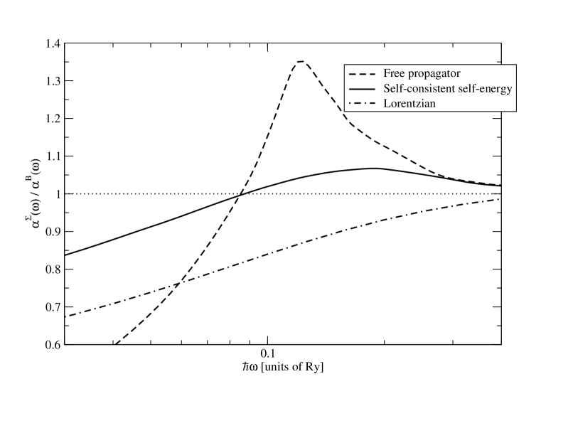
Figure 4: Correction factor $\alpha^{\mathrm{\Sigma}}(\omega)/\alpha^{\mathrm{\rm B}}(\omega)$ as a function of the photon energy $\hbar\omega$ with free propagators in self-energy diagram, the self-consistent spectral function, and a Lorentzian ansatz. Parameter values: Electron density $n_{\mathrm{e}}=10^{-6}a^{-3}_{\mathrm{B}}$, temperature $k_{\mathrm{B}}T=27.2\ \mathrm{eV}$  .

The result is shown in FIG. 4. The correction factor $\alpha^{\Sigma}(\omega)/\alpha^{\rm B}(\omega)$ (cf. Eq.(22)) is plotted as a function of the frequency for three different approximations with the parameters $n_{\mathrm{e}}=10^{-6}\,a_{\mathrm{B}}^{-3}$ and $k_{\mathrm{B}}T=27.2\ \mathrm{eV}$. The full line presents the result of the self-consistent treatment, Eq. (34), and is compared to a calculation with free propagators in the self-energy diagrams, see Eq. (29), and a calculation using a Lorentzian ansatz of the spectral function with a width taken at the on-shell energy $\Gamma(\boldsymbol{p},\hbar\omega=E^{\mathrm{e}}_{p})$. This corresponds to the introduction of a finite life-time in the approach of Knoll and Voskresensky knol:annals96 .

For the lowest frequencies considered here, all approximations show a suppression of the absorption coefficient as compared to the Born result. At high frequencies, all curves tend towards unity, i.e., the Born result is recovered. For intermediate frequencies, an enhancement of up to 35 % is found for the calculation using free propagators. Making use of the self consistency, the enhancement is reduced to 6 % at most. For the Lorentzian ansatz, no enhancement at all appears. Thus, the width of the imaginary part of the self-energy as a function of frequency $\omega$ (FIG. 3) plays a crucial rôle for the size of the enhancement. We expect that any increase in the width of the self-energy will further decrease the enhancement or even lead to a suppression for all frequencies as in the case of the Lorentzian ansatz, which corresponds to an infinite width of the imaginary part of the self-energy. A further broadening could result from an extension to higher orders in the set of diagrams for the self-consistent calculation of the spectral function, e.g. by inclusion of vertex terms.

III.4 D. Vertex corrections

As known from the Ward-Takahashi identities, self-energy and vertex corrections are intrinsically related. In particular, if medium corrections arise in a certain order of a small parameter like the density from the self-energy, also contributions from the vertex corrections are expected in the same order. This well-known fact is used to construct so-called conserved approximations kada:pr61 ; baym:pr62 and has also been discussed in the context of other medium effects, such as the modification of two-particle states or the inclusion of bound states into the polarization function and the calculation of optical line spectra profiles guen:habil . Thus, it is necessary to study the vertex corrections corresponding to the self-energy considered before. However, the solution of the vertex-equation is a technically very challenging task and has been solved so far only in certain approximations takada ; maha:prb94 . In lowest order, the vertex correction is obtained through insertion of one ion-loop inside the electron-loop:

$$G_{\dot{J}\dot{J}}^{\rm V}(\omega_{\mu})=\ \parbox{86.72267pt}{ \includegraphics[width=86.72267pt,clip]{eq_vert.eps}}~{}.$$ (43)

We find for the imaginary part of the force-force Green function

$${\rm Im}\,G^{\mathrm{V}}_{\dot{J}\dot{J}}(\omega+i\eta) = \frac{n_{\mathrm{i}}n_{\mathrm{e}}\Lambda_{\mathrm{e}}^{3}e^{6}}{24\pi^{3}\epsilon_{0}^{2}\hbar^{3}m_{\mathrm{e}}\omega}\bigg{[}\,\int\limits_{0}^{\infty}\mathrm{d}p\,p\,e^{-\beta\hbar^{2}p^{2}/2m_{\mathrm{e}}}\Gamma^{\mathrm{V}}(p)\ln\left|\frac{\sqrt{E^{\mathrm{e}}_{p}}+\sqrt{E^{\mathrm{e}}_{p}+\hbar\omega}}{\sqrt{E^{\mathrm{e}}_{p}}-\sqrt{E^{\mathrm{e}}_{p}+\hbar\omega}}\right|+$$ (44)

$$\qquad\qquad\ +\int\limits_{\sqrt{2m_{\mathrm{e}}\omega/\hbar}}^{\infty}\!\!\!\!\!\!\!\mathrm{d}p\,p\,{\rm e}^{-\beta\hbar^{2}p^{2}/2m_{\mathrm{e}}}\Gamma^{\mathrm{V}}(p)\ln\left|\frac{\sqrt{E^{\mathrm{e}}_{p}}+\sqrt{E^{\mathrm{e}}_{p}-\hbar\omega}}{\sqrt{E^{\mathrm{e}}_{p}}-\sqrt{E^{\mathrm{e}}_{p}-\hbar\omega}}\right|\bigg{]}~{},$$

with the vertex part

$$\Gamma^{\mathrm{V}}(p) = {\pi^{2}n_{\mathrm{i}}e^{4}m\over(2\pi)^{3}\hbar^{2}\epsilon_{0}^{2}\kappa p^{2}}~{},$$ (45)

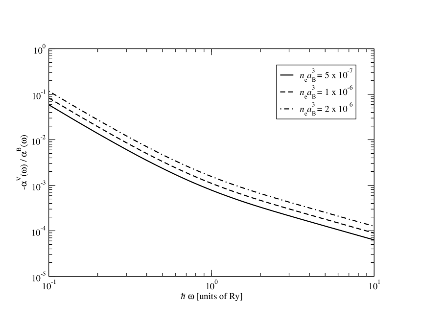
Figure 5: Correction factor $\alpha^{\mathrm{V}}(\omega)/\alpha^{\mathrm{\rm B}}(\omega)$ as a function of the photon energy $\hbar\omega$. For high energies the ratio behaves like $1/\omega$. Various values of the electron density are considered. Temperature: $k_{\mathrm{B}}T=27.2\ \mathrm{eV}$.

taken in lowest order in $\kappa$. For the details, see App. B. This expression can be evaluated numerically. In the limit of high frequencies, where the second integral becomes negligible compared to the first, the absorption coefficient is proportional to $K_{1}(\omega)/\omega^{4}$. Since the $K_{1}$ function has the same asymptotic behavior as the $K_{0}$ function, which was the characteristic of the Born result for the absorption coefficient Eq. (6), the ratio $\alpha^{\mathrm{V}}/\alpha^{\rm B}$ (cf. Eq. (22)) behaves like $1/\omega$ in the high frequency limit. The relative change of the absorption coefficient due to the vertex correction $\alpha^{\rm V}/\alpha^{\rm B}$ is shown in FIG. 5.

For all frequencies considered, a suppression with respect to the Born approximation is found. For the considered energy range, the corrections are small and decrease with increasing energy. For energies larger than 1 Ry, the expected high frequency behavior $\propto\omega^{-1}$ arises. The corrections are small for low densities compared to higher densities.

We consider the absorption coefficient $\alpha(\omega)$ including all of the improvements. Since the Born approximation is already included in the self-energy contribution $\alpha^{\Sigma}(\omega)$ we have

$$\alpha(\omega) = \alpha^{\rm V}(\omega)\,+\alpha^{\Sigma}(\omega)\;\;\;.$$ (46)

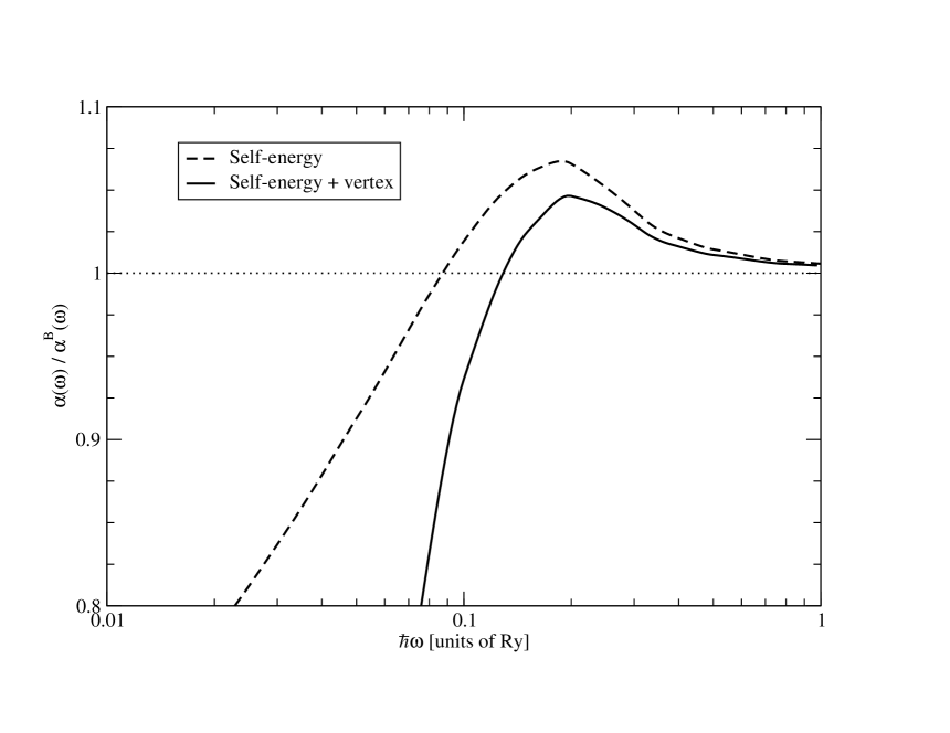
Figure 6: Total absorption coefficient taken relative to the Born result $\alpha^{\mathrm{V}}(\omega)/\alpha^{\mathrm{\rm B}}(\omega)$ as a function of the photon energy $\hbar\omega$. Parameter values: Electron density $n_{\mathrm{e}}=10^{-6}a^{-3}_{\mathrm{B}}$, temperature $k_{\mathrm{B}}T=27.2\ \mathrm{eV}$.

The relative change $\alpha(\omega)/\alpha^{\rm B}(\omega)$ is presented in FIG. 6. For the sake of comparison, the self-energy correction is shown as well. For small frequencies, the self-energy contribution and the vertex contribution add to a net suppression. For higher energies, the self-energy term shows an enhancement, which is partially compensated by the vertex. However, the net result is still an enhancement. In the high frequency limit, the Born result is reproduced.

IV 4. CONCLUSIONS

In this paper, we have studied the influence of the surrounding medium on the bremsstrahlung spectrum in non-ideal plasmas. The interaction with the medium leads to a finite life-time of the electron states. Instead of free quasi-particles, the spectral function has to be used to describe the electron properties in the medium. Thus, the use of the single-particle spectral function is a quantum-statistically sound implementation of the original idea of successive scatterings by Landau/Pomeranchuk and Migdal.

Our approach, namely the microscopic treatment of the dynamical self-energy, extends a recent work of Knoll and Voskresensky knol:annals96 , where a Lorentzian ansatz for the spectral function with a frequency-independent quasi-particle lifetime was considered. The Lorentzian ansatz for the spectral function was discussed above in subsection 3.C., taking the imaginary part of the self-energy at the quasi-particle energy. Then, a suppression of the bremsstrahlung spectrum was observed. In general, the microscopical treatment leads a frequency-dependent imaginary part of the self-energy, and, according to the Kramers-Kronig relation, to a non-vanishing real part. In particular, the inclusion of the real part of the self-energy in the spectral function influences the medium modification of the bremsstrahlung spectrum.

In the present paper, the one-loop approximation was taken for the self-energy. It has been shown that a self-consistent treatment has to be used in order to avoid unphysical artifacts which arise, if instead of the full propagator the free propagator is taken to evaluate the self-energy. This is already known from the treatment of the spectral functions in plasma physics in the so-called GW approximation maha where the interaction with the medium is implemented by a screened potential. It should be mentioned that in this case a self-consistent treatment of the spectral function on the level of the GW approximation has been performed WR . Any iterative solution starting from the free propagator leads to non-physical structures in the spectral function, see also fehr .

Within our approach, we found a switch from a suppression at low frequencies to an enhancement at high frequencies for the bremsstrahlung spectrum. The approximation for the self-energy can be improved by considering further diagrams. In particular, the vertex correction would be of interest which modifies the coupling to the interaction potential. The inclusion of vertex corrections is also necessary to obtain conserved approximations and has been shown in Subsection 3.D., where a further suppression of the bremsstrahlung spectrum was observed. In conclusion, the modification of the bremsstrahlung spectrum by the surrounding medium is sensitively dependent on the approximation used.

We cannot elaborate further on the switch from suppression to enhancement seen in the self-energy correction. In order to verify the existence of such a switch, higher order calculations are necessary. A consistent procedure would consist in a) using the full propagator in the calculation of the vertex correction, b) solving the full vertex equation with full propagators and finally c) solve the Dyson equation for the single particle propagator with the solution of the vertex equation.

The importance of vertex corrections in the self consistency relations has also been shown in the description of the spectral function of the homogeneous electron gas. There, notable differences between a so-called GW$\Gamma$ approximation takada including vertex terms and a GW approximation holm arise. It should be mentioned that self-consistent Schwinger-Dyson equations for the self-energy have been considered in field theory Craig to find solutions for the QCD running coupling problem. A corresponding treatment would lead to a better description of the modification of the bremsstrahlung spectrum in a dense medium, but would exceed the frame of the present work. Also, at low frequencies, further effects such as the dielectric suppression are of importance. It has not been considered in this approach, but can easily be obtained from the force-force correlation function as well.

V ACKNOWLEDGEMENTS

We would like to thank J. Knoll, D. Voskresensky and V. Morozov for stimulating discussions. C.F. would also like to thank the Gesellschaft für Schwerionenforschung (GSI) for its hospitality and the Studienstiftung des Deutschen Volkes for a scholarship.

Appendix A APPENDIX A: Details on the Born approximation

The four-particle Green function $G_{\dot{J}\dot{J}}$ in Born approximation is given by

$$G^{\mathrm{Born}}_{\dot{J}\dot{J}}(\omega_{\mu}) = \frac{e^{2}}{m_{\mathrm{e}}^{2}\Omega_{0}^{2}}\sum_{\boldsymbol{pkq}\atop\omega_{\lambda},z_{\nu},z_{\bar{\nu}}}\left|v_{q}^{\rm ei}\right|^{2}q_{z}^{2}\frac{1}{z_{\nu}-E_{k}^{\rm i}}\,\frac{1}{z_{\nu}-\omega_{\lambda}-E_{k-q}^{\rm i}}\,\frac{1}{z_{\bar{\nu}}-E^{\rm e}_{p}}\,\frac{1}{z_{\bar{\nu}}+\omega_{\mu}+\omega_{\lambda}-E_{p+q}^{\rm e}}\;\;\;.$$ (A1)

Here, $z_{\nu},z_{\bar{\nu}}$ denote Fermionic Matsubara frequencies, while $\omega_{\mu},\omega_{\lambda}$ are Bosonic Matsubara frequencies. We use the convention $z_{\nu}=(2\nu+1)\pi i/\beta+\mu_{c},\,\nu=0,\pm 1,\pm 2,\ldots$ and $\omega_{\lambda}=2\lambda\pi i/\beta,\,\lambda=0,\pm 1,\pm 2,\ldots$. $\mu_{c}$ is the chemical potential of a particle of species $c$. We refer to Ref. krae for details concerning thermodynamic Green functions. The summation over $z_{\nu},z_{\bar{\nu}},\omega_{\lambda}$ can be carried out analytically.

In the adiabatic approximation the summation over $z_{\bar{\nu}}$ and $k$ gives the ionic density $n_{\mathrm{i}}$. After summation of $z_{\nu}$ we have

$$G^{\mathrm{Born}}_{\dot{J}\dot{J}}(\omega_{\mu})={n_{\mathrm{i}}e^{2}\over m_{\mathrm{e}}^{2}\Omega_{0}}\sum_{\boldsymbol{pq}}|v^{\mathrm{ei}}_{q}|^{2}q_{z}^{2}\frac{f(E^{\mathrm{e}}_{p})-f(E^{\mathrm{e}}_{p+q})}{E^{\mathrm{e}}_{p}+\omega_{\mu}-E^{\mathrm{e}}_{p+q}}~{},$$ (A2)

and by virtue of the Dirac identity we obtain after analytic continuation

$${\rm Im}\,G^{\mathrm{Born}}_{\dot{J}\dot{J}}(\omega+i\eta)=-{\pi n_{\rm i}e^{2}\over m_{\mathrm{e}}^{2}\Omega_{0}}\sum_{\boldsymbol{pq}}|v^{\mathrm{ei}}_{q}|^{2}q_{z}^{2}\left[f(E^{\mathrm{e}}_{p})-f(E^{\mathrm{e}}_{p+q})\right]\delta(\hbar\omega+E^{\mathrm{e}}_{p}-E^{\mathrm{e}}_{p+q})\ .$$ (A3)

Replacing the sums over momenta by integrals and assuming a Maxwellian plasma, we find

$${\rm Im}\,G^{\mathrm{Born}}_{\dot{J}\dot{J}} = \frac{\pi n_{\mathrm{i}}n_{\mathrm{e}}\Lambda_{\mathrm{e}}^{3}e^{2}}{m_{\mathrm{e}}(2\pi)^{6}}\frac{1-\mathrm{\rm e}^{-\beta\hbar\omega}}{(\hbar\omega)^{2}}\int\limits_{0}^{\infty}\mathrm{d}p\,p\,4\pi\,\mathrm{e}^{-\beta\hbar^{2}p^{2}/2m_{\mathrm{e}}}\!\!\int\limits_{0}^{\infty}\mathrm{d}q\,2\pi{q^{3}\over 3}\left({e^{2}\over\epsilon_{0}\Omega_{0}(q^{2}+\kappa^{2})}\right)^{2}\int\limits_{-1}^{1}\mathrm{d}z\,\delta(z-{m_{\mathrm{e}}\omega\over\hbar pq}+{q\over 2p})~{}.$$

The limits of the $q$-integration are obtained from the root of the argument of the delta function, $p\geq\left|{m_{\mathrm{e}}\omega\over\hbar q}-{q\over 2}\right|$ or equivalently $-p+\sqrt{p^{2}+2m_{\mathrm{e}}\omega/\hbar}\leq q\leq p+\sqrt{p^{2}+2m_{\mathrm{e}}\omega/\hbar}$. Performing the integrations first over $q$ and then over $p$, we obtain the result Eq.(25).

Appendix B APPENDIX B: Details on the vertex correction

The vertex contribution to the force-force Green function is given by

$$G^{\mathrm{V}}_{\dot{J}\dot{J}}(\omega_{\mu})={e^{2}\over m^{2}\Omega_{0}^{2}}\sum_{\boldsymbol{pkqk^{\prime}q^{\prime}}\atop z_{\nu}z_{\mu}z_{\mu}^{\prime}\omega_{\lambda}\omega_{\lambda}^{\prime}}|v_{q}^{\rm ei}|^{2}q_{z}^{2}|v^{\rm ei}_{q^{\prime}}|^{2}{1\over z_{\mu}-E^{\mathrm{i}}_{k}}{1\over z_{\mu}-\omega_{\lambda}-E^{\mathrm{i}}_{k-q}}{1\over z_{\nu}-E^{\mathrm{e}}_{p}}{1\over z_{\nu}+\omega_{\mu}+\omega_{\lambda}-E^{\mathrm{e}}_{p+q}}\times$$

$$\qquad\qquad\qquad\times{1\over z_{\mu}^{\prime}-E^{\mathrm{i}}_{k^{\prime}}}{1\over z_{\mu}^{\prime}-\omega_{\lambda}^{\prime}-E^{\mathrm{i}}_{k^{\prime}-q^{\prime}}}{1\over z_{\nu}+\omega_{\mu}+\omega_{\lambda}+\omega_{\lambda}^{\prime}-E^{\mathrm{e}}_{p+q+q^{\prime}}}{1\over z_{\nu}+\omega_{\lambda}^{\prime}-E^{\mathrm{e}}_{p+q^{\prime}}}~{}.$$ (B1)

Again, summation over ionic variables $z_{\mu},z^{\prime}_{\mu},k,k^{\prime}$ and bosonic frequencies $\omega_{\lambda}$ and $\omega^{\prime}_{\lambda}$ can be performed, which gives in adiabatic approximation the ion density $n_{\mathrm{i}}$. Thus,

$$G^{\mathrm{V}}_{\dot{J}\dot{J}}(\omega_{\mu})=\frac{e^{2}}{m^{2}\Omega^{2}_{0}}n_{\mathrm{i}}^{2}\sum_{\boldsymbol{pqq^{\prime}},z_{\nu}}|v_{q}^{\rm ei}|^{2}q_{z}^{2}|v^{\mathrm{ei}}_{q^{\prime}}|^{2}{1\over z_{\nu}-E^{\mathrm{e}}_{p}}{1\over z_{\nu}+\omega_{\mu}-E^{\mathrm{e}}_{p+q}}{1\over z_{\nu}+\omega_{\mu}-E^{\mathrm{e}}_{p+q+q^{\prime}}}{1\over z_{\nu}-E^{\mathrm{e}}_{p+q^{\prime}}}~{}.$$ (B2)

Expansion into partial fractions with respect to $z_{\nu}$ and summation leads to

$$G^{\mathrm{V}}_{\dot{J}\dot{J}}(\omega_{\mu}) = n_{\mathrm{i}}^{2}\sum_{\boldsymbol{pqq^{\prime}}}|v_{q}^{\rm ei}|^{2}q_{z}^{2}|v^{\mathrm{ei}}_{q^{\prime}}|^{2}\Big{\{}f(E^{\mathrm{e}}_{p+q}){1\over E^{\mathrm{e}}_{p+q}-\omega_{\mu}-E^{\mathrm{e}}_{p}}{1\over E^{\mathrm{e}}_{p+q}-\omega_{\mu}-E^{\mathrm{e}}_{p+q^{\prime}}}{1\over E^{\mathrm{e}}_{p+q}-E^{\mathrm{e}}_{p+q+q^{\prime}}}$$ (B3)

$$+f(E^{\mathrm{e}}_{p}){1\over E^{\mathrm{e}}_{p}+\omega_{\mu}-E^{\mathrm{e}}_{p+q}}{1\over E^{\mathrm{e}}_{p}+\omega_{\mu}-E^{\mathrm{e}}_{p+q+q^{\prime}}}{1\over E^{\mathrm{e}}_{p}-E^{\mathrm{e}}_{p+q^{\prime}}}+$$

$$+f(E^{\mathrm{e}}_{p+q^{\prime}}){1\over E^{\mathrm{e}}_{p+q^{\prime}}+\omega_{\mu}-E^{\mathrm{e}}_{p+q}}{1\over E^{\mathrm{e}}_{p+q^{\prime}}+\omega_{\mu}-E^{\mathrm{e}}_{p+q+q^{\prime}}}{1\over E^{\mathrm{e}}_{p+q^{\prime}}-E^{\mathrm{e}}_{p}}$$

$$+f(E^{\mathrm{e}}_{p+q+q^{\prime}}){1\over E^{\mathrm{e}}_{p+q+q^{\prime}}-\omega_{\mu}-E^{\mathrm{e}}_{p}}{1\over E^{\mathrm{e}}_{p+q+q^{\prime}}-\omega_{\mu}-E^{\mathrm{e}}_{p+q^{\prime}}}{1\over E^{\mathrm{e}}_{p+q+q^{\prime}}-E^{\mathrm{e}}_{p+q}}\Big{\}}~{}.$$

Rigorously, one would have to perform another expansion into partial fractions in order to obtain the imaginary part of this Green function. This procedure would lead to delta functions of the form $\delta(E^{\mathrm{e}}_{p}-E^{\mathrm{e}}_{p+q})$ without a bosonic frequency of the external field in the argument. These are residues of a perturbation expansion of the wave functions of the electron in the ion’s potential and do not yield any information about the dynamics of the system. Thus, only those denominators in Eq.(B3) are of interest, that do contain the frequency $\omega_{\mu}$. It suffices to perform an expansion into partial fractions with respect to $\omega_{\mu}$. We obtain

$$\mathrm{Im}\,G^{\mathrm{V}}_{\dot{J}\dot{J}}(\omega) = n_{\mathrm{i}}^{2}\pi\sum_{\boldsymbol{pqq^{\prime}}}|v_{q}^{\rm ei}|^{2}q_{z}^{2}|v^{\mathrm{ei}}_{q^{\prime}}|^{2}\Big{[}-f(E^{\mathrm{e}}_{p+q})\ \delta(\hbar\omega+E^{\mathrm{e}}_{p}-E^{\mathrm{e}}_{p+q}){1\over E^{\mathrm{e}}_{p}-E^{\mathrm{e}}_{p+q^{\prime}}}{1\over E^{\mathrm{e}}_{p+q}-E^{\mathrm{e}}_{p+q+q^{\prime}}}-$$ (B4)

$$-f(E^{\mathrm{e}}_{p+q})\ \delta(\hbar\omega+E^{\mathrm{e}}_{p+q^{\prime}}-E^{\mathrm{e}}_{p+q}){1\over E^{\mathrm{e}}_{p+q^{\prime}}-E^{\mathrm{e}}_{p}}{1\over E^{\mathrm{e}}_{p+q}-E^{\mathrm{e}}_{p+q+q^{\prime}}}+$$

$$+f(E^{\mathrm{e}}_{p})\ \delta(\hbar\omega+E^{\mathrm{e}}_{p}-E^{\mathrm{e}}_{p+q}){1\over E^{\mathrm{e}}_{p}-E^{\mathrm{e}}_{p+q^{\prime}}}{1\over E^{\mathrm{e}}_{p+q}-E^{\mathrm{e}}_{p+q+q^{\prime}}}+$$

$$+f(E^{\mathrm{e}}_{p})\ \delta(\hbar\omega+E^{\mathrm{e}}_{p}-E^{\mathrm{e}}_{p+q+q^{\prime}}){1\over E^{\mathrm{e}}_{p}-E^{\mathrm{e}}_{p+q^{\prime}}}{1\over E^{\mathrm{e}}_{p+q+q^{\prime}}-E^{\mathrm{e}}_{p+q}}+$$

$$+f(E^{\mathrm{e}}_{p+q^{\prime}})\ \delta(\hbar\omega+E^{\mathrm{e}}_{p+q^{\prime}}-E^{\mathrm{e}}_{p+q}){1\over E^{\mathrm{e}}_{p+q^{\prime}}-E^{\mathrm{e}}_{p}}{1\over E^{\mathrm{e}}_{p+q}-E^{\mathrm{e}}_{p+q+q^{\prime}}}+$$

$$+f(E^{\mathrm{e}}_{p+q^{\prime}})\ \delta(\hbar\omega+E^{\mathrm{e}}_{p+q^{\prime}}-E^{\mathrm{e}}_{p+q+q^{\prime}}){1\over E^{\mathrm{e}}_{p+q^{\prime}}-E^{\mathrm{e}}_{p}}{1\over E^{\mathrm{e}}_{p+q+q^{\prime}}-E^{\mathrm{e}}_{p+q}}-$$

$$-f(E^{\mathrm{e}}_{p+q+q^{\prime}})\ \delta(\hbar\omega+E^{\mathrm{e}}_{p}-E^{\mathrm{e}}_{p+q+q^{\prime}}){1\over E^{\mathrm{e}}_{p+q+q^{\prime}}-E^{\mathrm{e}}_{p+q}}{1\over E^{\mathrm{e}}_{p}-E^{\mathrm{e}}_{p+q^{\prime}}}-$$

$$-f(E^{\mathrm{e}}_{p+q+q^{\prime}})\ \delta(\hbar\omega+E^{\mathrm{e}}_{p+q^{\prime}}-E^{\mathrm{e}}_{p+q+q^{\prime}}){1\over E^{\mathrm{e}}_{p+q+q^{\prime}}-E^{\mathrm{e}}_{p+q}}{1\over E^{\mathrm{e}}_{p+q^{\prime}}-E^{\mathrm{e}}_{p}}\Big{]}~{}.$$

This can be cast into the form

$${\rm Im}\,G^{\mathrm{V}}_{\dot{J}\dot{J}}(\omega+i\eta)=n_{\mathrm{i}}^{2}\pi\sum_{\boldsymbol{pqq^{\prime}}}|v_{q}^{\rm ei}|^{2}q_{z}^{2}|v^{\mathrm{ei}}_{q^{\prime}}|^{2}f(E^{\mathrm{e}}_{p}){1\over E^{\mathrm{e}}_{p}-E^{\mathrm{e}}_{p+q^{\prime}}}{1\over E^{\mathrm{e}}_{p+q}-E^{\mathrm{e}}_{p+q+q^{\prime}}}\times$$

$$\times\left[\delta(\hbar\omega+E^{\mathrm{e}}_{p}-E^{\mathrm{e}}_{p+q})-\delta(\hbar\omega+E^{\mathrm{e}}_{p}-E^{\mathrm{e}}_{p+q+q^{\prime}})-\delta(\hbar\omega-E^{\mathrm{e}}_{p}+E^{\mathrm{e}}_{p+q})+\delta(\hbar\omega-E^{\mathrm{e}}_{p}+E^{\mathrm{e}}_{p+q+q^{\prime}})\right]~{},$$ (B5)

where only the distribution function $f(E^{\mathrm{e}}_{p})$ appears.
For small internal momenta $q^{\prime}$ the denominator $E^{\mathrm{e}}_{p+q}-E^{\mathrm{e}}_{p+q+q^{\prime}}$ can be expanded and vanishes after rewriting the delta function as $\delta(\hbar\omega+E^{\mathrm{e}}_{p}-E^{\mathrm{e}}_{p+q+q^{\prime}})=\delta(\hbar\omega+E^{\mathrm{e}}_{p}-E^{\mathrm{e}}_{p+q}+E^{\mathrm{e}}_{p+q}-E^{\mathrm{e}}_{p+q+q^{\prime}})$. For $\omega\to 0$, this argument does not hold, but it is used here in order to find the influence of the vertex correction at finite frequencies $\omega$.
Eq. (B5) becomes

$${\rm Im}\,G^{\mathrm{V}}_{\dot{J}\dot{J}}(\omega+i\eta) = {\mathrm{d}\over\mathrm{d}\omega}2\,n_{\rm i}^{2}\pi\sum_{\boldsymbol{pqq^{\prime}}}|v_{q}^{\rm ei}|^{2}q_{z}^{2}|v^{\mathrm{ei}}_{q^{\prime}}|^{2}f(E^{\mathrm{e}}_{p}){1\over E^{\mathrm{e}}_{p}-E^{\mathrm{e}}_{p+q^{\prime}}}\times$$ (B6)

$$\times\left[\delta(\hbar\omega+E^{\mathrm{e}}_{p}-E^{\mathrm{e}}_{p+q})-\delta(\hbar\omega-E^{\mathrm{e}}_{p}+E^{\mathrm{e}}_{p+q})\right]~{}.$$

Replacing the summation over the momenta by an integration, we have

$${\rm Im}\,G^{\mathrm{V}}_{\dot{J}\dot{J}}(\omega+i\eta)=\frac{\mathrm{d}}{\mathrm{d}\omega}{2n_{\mathrm{i}}^{2}\pi\over\hbar^{2}}\int{\mathrm{d}^{3}p\over(2\pi)^{3}}\int{\mathrm{d}^{3}q\over(2\pi)^{3}}\int{\mathrm{d}^{3}q^{\prime}\over(2\pi)^{3}}|v_{q}^{\rm ei}|^{2}q_{z}^{2}|v^{\mathrm{ei}}_{q^{\prime}}|^{2}f(E^{\mathrm{e}}_{p}){m_{\mathrm{e}}\over\boldsymbol{p}\cdot\boldsymbol{q}^{\prime}+q^{\prime 2}/2}\times$$

$$\times\{\delta(\hbar\omega-\boldsymbol{p}\cdot\boldsymbol{q}/m_{\mathrm{e}}-q^{2}/2m_{\mathrm{e}})-\delta(\hbar\omega+\boldsymbol{p}\cdot\boldsymbol{q}/m_{\mathrm{e}}+q^{2}/2m_{\mathrm{e}})\}~{}.$$ (B7)

Comparing Eq.(B7) to the Born result Eq.(LABEL:eqn:born_101), an additional function arises

$$\Gamma^{\mathrm{V}}(p) = {2n_{\mathrm{i}}\Omega_{0}^{2}\over(2\pi)^{3}\hbar^{2}}\int\mathrm{d}^{3}q^{\prime}|v^{\mathrm{ei}}_{q^{\prime}}|^{2}{m_{\mathrm{e}}\over\boldsymbol{p}\cdot\boldsymbol{q}^{\prime}+q^{\prime 2}/2}={4\pi e^{4}n_{\mathrm{i}}m_{\mathrm{e}}\over(2\pi)^{3}\hbar^{2}\epsilon_{0}^{2}p}\int_{0}^{\infty}\!\mathrm{d}q^{\prime}{q^{\prime}\over(q^{\prime 2}+\kappa^{2})^{2}}\int\limits_{-1}^{1}\!\mathrm{d}z{1\over z+q^{\prime}/2p}$$ (B8)

$$= {4\pi n_{\mathrm{i}}e^{4}m_{\mathrm{e}}\over(2\pi)^{3}\hbar^{2}\epsilon_{0}^{2}p}\int_{0}^{\infty}\!\mathrm{d}q^{\prime}{q^{\prime}\over(q^{\prime 2}+\kappa^{2})^{2}}\ln\left|{1+q^{\prime}/2p\over 1-q^{\prime}/2p}\right|={4\pi^{2}n_{\mathrm{i}}e^{4}m_{\mathrm{e}}\over(2\pi)^{3}\hbar^{2}\epsilon_{0}^{2}}{1\over 4p^{2}\kappa+\kappa^{3}}\;\;\;,$$

which is obtained from the integration over $q^{\prime}$. The $q$ integration can be performed as above, cf. Eq. (25). Insertion into the force-force correlation function Eq.(19) gives

$$\big{\langle}\,\,\dot{\!\!J}_{0}^{z},\,\,\dot{\!\!J}_{0}^{z}\big{\rangle}_{\omega+i\eta}^{\rm V} = {ie^{2}\hbar\pi\over\beta\Omega_{0}^{3}m_{\mathrm{e}}^{2}}\int{\mathrm{d}\hbar\bar{\omega}\over\pi}{1\over\omega-\bar{\omega}+i\eta}{1\over\hbar\bar{\omega}}{\mathrm{d}\over\mathrm{d}\hbar\bar{\omega}}\sum_{\boldsymbol{pq}}|v_{q}^{\rm ei}|^{2}{q^{2}\over 3}f(E^{\mathrm{e}}_{p})n_{\rm i}\Gamma^{\rm V}(p)\times$$ (B9)

$$\qquad\times\left[\delta(\hbar\bar{\omega}-{\hbar^{2}pqz\over m_{\mathrm{e}}}-{\hbar^{2}q^{2}\over 2m_{\mathrm{e}}})+\delta(-\hbar\bar{\omega}-{\hbar^{2}pqz\over m_{\mathrm{e}}}-{\hbar^{2}q^{2}\over 2m_{\mathrm{e}}})\right]~{}.$$

Through partial integration we obtain the simple pôle-structure

$$\big{\langle}\,\,\dot{\!\!J}_{0}^{z},\,\,\dot{\!\!J}_{0}^{z}\big{\rangle}_{\omega+i\eta}^{\rm V}={ie^{2}\hbar\over\beta\Omega_{0}^{3}m_{\mathrm{e}}^{2}}\sum_{\boldsymbol{pq}}|v_{q}^{\rm ei}|^{2}{q^{2}\over 3}f(E^{\mathrm{e}}_{p})n_{\mathrm{i}}\Gamma^{\rm V}(p){1\over(E^{\mathrm{e}}_{p}-E^{\mathrm{e}}_{p+q})^{2}}\left[{1\over\hbar\omega+i\eta-{\hbar^{2}pqz\over m_{\mathrm{e}}}-{\hbar^{2}q^{2}\over 2m}}+{1\over\hbar\omega+i\eta+{\hbar^{2}pqz\over m_{\mathrm{e}}}+{\hbar^{2}q^{2}\over 2m_{\mathrm{e}}}}\right]\;,$$ (B10)

and thereby

$${\rm Re}\,\big{\langle}\,\,\dot{\!\!J}_{0}^{z},\,\,\dot{\!\!J}_{0}^{z}\big{\rangle}_{\omega+i\eta}^{\rm V}={e^{2}\hbar\over\beta\Omega_{0}m_{\mathrm{e}}^{2}}{n_{\mathrm{i}}\pi\over(\hbar\omega)^{2}}\sum_{\boldsymbol{pq}}|v_{q}^{\rm ei}|^{2}{q^{2}\over 3}f(E^{\mathrm{e}}_{p})\Gamma^{\rm V}(p)\left[\delta(\hbar\omega-{\hbar^{2}pqz\over m_{\mathrm{e}}}-{\hbar^{2}q^{2}\over 2m_{\mathrm{e}}})+\delta(\hbar\omega+{\hbar^{2}pqz\over m_{\mathrm{e}}}+{\hbar^{2}q^{2}\over 2m_{\mathrm{e}}})\right]$$

$$={e^{6}\over\epsilon_{0}^{2}\beta\hbar m_{\mathrm{e}}}{1\over(\hbar\omega)^{2}}{n_{\mathrm{i}}n_{\mathrm{e}}\Lambda_{\mathrm{e}}^{3}\over 24\pi^{3}\Omega_{0}}\int_{0}^{\infty}\!\mathrm{d}p\,p\,\mathrm{e}^{-\beta\hbar^{2}p^{2}/2m_{\mathrm{e}}}\Gamma^{\rm V}(p)\int_{0}^{\infty}\!\mathrm{d}q\,{q^{3}\over(q^{2}+\kappa^{2})^{2}}\int\limits_{-1}^{1}\mathrm{d}z\left[\delta(z+{q\over 2p}-{m_{\mathrm{e}}\omega\over\hbar pq})+\delta(z+{q\over 2p}+{m_{\mathrm{e}}\omega\over\hbar pq})\right]~{}.$$

The corresponding Green function $G_{\dot{J}\dot{J}}(\omega_{\mu})$ evaluates to Eq. (44).

Figure 1: Diagrammatic representation of $G_{\dot{J}\dot{J}}(\omega_{\mu})$. (a) full account of all medium effects by a four particle Green function,
(b) factorization into two polarization bubbles, (c) Born approximation.

Figure 3: Imaginary and real part of the electrons self-energy $\Sigma_{\mathrm{e}}(p,\hbar\omega)$, dispersion relation, and spectral function $A_{\mathrm{e}}(p,\hbar\omega)$ for $p=1~{}a_{\mathrm{B}}^{-1}$ (a) from self-consistent calculation cf. Eq. (34) and (b) using free propagators, cf. Eq. (37). The parameters are: Electron density $n_{\mathrm{e}}=10^{-6}a^{-3}_{\mathrm{B}}$, temperature $k_{\mathrm{B}}T=27.2\ \mathrm{eV}$.

References

- (1) H. R. Griem, Principles of Plasma Spectroscopy (Cambridge University Press, Cambridge, 1997).
- (2) C. Itzykson and J.-B. Zuber, Quantum field theory (McGraw-Hill, New York, 1980).
- (3) H. Bethe and W. Heitler, Proc. Roy. Soc. A 146, 83 (1934).
- (4) W. Heitler, The Quantum Theory of Radiation (Oxford University Press, Oxford, 1957).
- (5) B. R. Holstein, Topics in Advanced Quantum Mechanics (Addison-Wesley, Redwood, 1992).
- (6) J. D. Bjorken and D. Drell, Relativistic Quantum Fields (McGraw-Hill, New York, 1965).
- (7) A. Sommerfeld, Atombau und Spektrallinien (Vieweg-Verlag, Braunschweig, 1949).
- (8) G. Elwert, Ann. Phys. 34, 178 (1939).
- (9) H. A. Kramers, Phil. Mag. 46, 836 (1923).
- (10) G. Bekefi, Radiation Processes in Plasmas (Wiley, New York, 1966).
- (11) H. Reinholz, R. Redmer, G. Röpke, and A. Wierling, Phys. Rev. E 62, 5648 (2000).
- (12) A. Wierling, Th. Millat, G. Röpke, and R. Redmer, Phys. Plasma 8, 3810 (2001).
- (13) L. D. Landau and I. J. Pomeranchuk, Dokl. Akad. Nauk SSSR 92, 535 (1953).
- (14) A. B. Migdal, Phys. Rev. 103, 1811 (1956).
- (15) B. G. Zakharov, JETP Lett. 63, 952 (1996).
- (16) B. G. Zakharov, JETP Lett. 64, 781 (1996).
- (17) A. V. Koshelkin, J. Phys. A 35, 8763 (2002).
- (18) S. Klein, Rev. Mod. Phys. 71, 1501 (1999).
- (19) E. Wang, J. Phys. G 27, 2379 (2001).
- (20) M. Czachor, Phys. Lett. A 313, 380 (2003).
- (21) A. A. Varfolomeev et al., Sov. Phys. JETP 11, 23 (1960).
- (22) E. Lohrmann, Phys. Rev. 122, 1908 (1961) .
- (23) P. H. Fowler, D. H. Perkins, and K. Pinkau, Phil. Mag. 4, 1030 (1959).
- (24) K. Kasahara, Phys. Rev. D 31, 2737 (1985).
- (25) S. C. Strausz et al., Proc. of the 22nd Intl. Cosmic Ray Conf. 4, 233 (1991).
- (26) A. A. Varfolomeev et al., Sov. Phys. JETP 42, 218 (1975).
- (27) P. L. Anthony et al., Phys. Rev. D 56, 1373 (1997).
- (28) J. F. Bak, Nucl. Phys. B 302, 525 (1988).
- (29) H. D. Hansen et al., Phys. Rev. Lett. 91, 014801 (2003).
- (30) H. D. Hansen et al., Phys. Rev. D 69, 032001 (2004).
- (31) J. Knoll and D. Voskresensky, Ann. Phys. 249, 532 (1996).
- (32) D. Voskresensky, private communication (2003).
- (33) W. D. Kraeft, D. Kremp, W. Ebeling, and G. Röpke, Quantum Statistics of Charged Particle Systems (Akademie-Verlag, Berlin, 1986).
- (34) J. D. Jackson, Classical Electrodynamics (Wiley & Sons, New York, 1975), 2. edition.
- (35) G. D. Mahan, Many-Particle Physics (Plenum Press, New York and London, 1981), 2. edition.
- (36) M. L. Ter-Mikaelyan, Dokl. Akad. Nauk SSSR 94, 1033 (1953).
- (37) D. Zubarev, V. Morozov, and G. Röpke, Statistical Mechanics of Nonequilibrium Processes (Akademie-Verlag, Berlin, 1996), Vol. 2.
- (38) I. H. Hutchinson, Principles of Plasma Diagnostics (Cambridge University Press, Cambridge, 1987).
- (39) G. Baym and L. Kadanoff, Phys. Rev. 124, 287 (1961).
- (40) G. Baym, Phys. Rev 127, 1391 (1962).
- (41) S. Günter, Habilitation thesis, Rostock 1995
- (42) Y. Takada, Phys. Rev. Lett. 87, 226402 (2001).
- (43) S. Hong and G. D. Mahan, Phys. Rev. B 50, 8182 (1994).
- (44) A. Wierling and G. Röpke, Contrib. Plasma Phys. 38, 513 (1998).
- (45) R. Fehr, Ph.D. thesis, Greifswald, 1997.
- (46) B. Holm, Phys. Rev. Lett. 83, 788 (1999).
- (47) C. D. Roberts and S. M. Schmidt, Prog. Part. Nucl. Phys. 45, S1 (2000).