The occupation of a box
as a toy model for the seismic cycle of a fault

Abstract

We illustrate how a simple statistical model can describe the quasiperiodic occurrence of large earthquakes. The model idealizes the loading of elastic energy in a seismic fault by the stochastic filling of a box. The emptying of the box after it is full is analogous to the generation of a large earthquake in which the fault relaxes after having been loaded to its failure threshold. The duration of the filling process is analogous to the seismic cycle, the time interval between two successive large earthquakes in a particular fault. The simplicity of the model enables us to derive the statistical distribution of its seismic cycle. We use this distribution to fit the series of earthquakes with magnitude around 6 that occurred at the Parkfield segment of the San Andreas fault in California. Using this fit, we estimate the probability of the next large earthquake at Parkfield and devise a simple forecasting strategy.

American Journal of Physics, Vol. 73, No. 10, October 2005, pp. 946-952. DOI: 10.1119/1.2013310

I Introduction

In reporting the mechanism of the great California earthquake of 1906, ReidReid presented the elastic rebound theory. It assumes that an earthquake is the result of a sudden relaxation of elastic strain by rupture along a fault (a rupture surface between two rock blocks that move past each other). This theory extended earlier insights into the relation between earthquakes and faults by other geologists,Yeats especially Gilbert,Gilbert ; Gilbert506 McKay,McKay and Koto.Koto Since its formulation, it has been the basis for interpreting the earthquakes that occur in faults in the Earth’s upper, fragile crust.

According to Reid’s theory, elastic energy slowly accumulates on a fault over a long time after the occurrence of an earthquake, as the rock blocks on both sides of the fault are strained by tectonic forces. When the strain is large enough, the system relaxes by fast rupture and/or frictional sliding along the fault during the next earthquake. The elastic waves generated by this sudden event are the seismic waves that seismometers detect.

The tectonic loading and relaxation process of a fault is cyclic. The seismic cycle is the time interval between two successive large earthquakes on the same fault, frequently called characteristic earthquakes.Schwartz60 If the seismic cycle were periodic, earthquake prediction would be easy. There is increasing information about earthquake occurrences in the seismic record, compiled with historical data and recognition of ancient large earthquakes on faults.Yeats These data show that the seismic cycle of any given fault is not strictly periodic. The reason is that the tectonic loading and relaxation of a fault are complex nonlinear processes.GeoComplexity Moreover, faults occur in topologically complex networks,Bonnet343 and an earthquake occurring in a fault influences what occurs in other faults.Harris366

The duration of the seismic cycle is not constant, but follows a statistical distribution that can be empirically deduced from the earthquake time series.Savage540 This distribution, if it were known, could be used to estimate the probability of the next earthquake. However, it is not well known, because there are little data (typically less than ten) in the earthquake time series for any given fault or fault segment.Savage540 To use this probabilistic approach, it is convenient to fit the data to a theoretical statistical distribution.

Especially since the 1970s,VereJones ; Utsu0 ; Utsu1 ; Rikitake504 ; Hagiwara505 ; Rikitake ; VereJones2 earthquake recurrence is frequently considered as a renewal process,Cinlar ; Daley in which the times between successive events, in this case the large earthquakes in a fault, are assumed to be independent and identically distributed random variables. In this interpretation, the expected time of the next event does not depend on the details of the last event, except the time it occurred. In combination with elastic rebound theory, the probability of another earthquake would be low just after a fault-rupturing earthquake, and would then gradually increase, as tectonic deformation slowly stresses the fault again. When an earthquake finally occurs, it resets the renewal process to its initial state. Several well-known statistical distributions (such as the gamma,Utsu497 log-normal,Nishenko464 and WeibullHagiwara505 ; Utsu497 ; Kiremidjian315 ; Sieh ) have been used to describe the duration of the seismic cycle and to calculate the conditional probabilities of future earthquakes. These distributions also have been used as failure models for reliability and time-to-failure problems.Mann

More recently, many numerical models have been devised for simulating the tectonic processes occurring on a seismic fault.Main296 ; BenZion493 These models can generate as many synthetic earthquakes as desired,Ward542 so the statistical distribution of the time intervals between them can be fully characterized.Robinson608 Two highly idealized models are the Brownian passage time model,Matthews and the minimalist model.VazquezPrada250 ; Vazquez2 ; Gomez&Pacheco546 Their seismic cycle distributions have been used as renewal models, to fit actual earthquake series and estimate future earthquake probabilities. Matthews ; Gomez&Pacheco546 ; Gonzalez They, as well as the gamma, log-normal and Weibull distributions, provide a reasonably good fit to the existing data.Utsu497 ; Gomez&Pacheco546 ; Gonzalez The renewal models have been widely applied, particularly in JapanImoto472 and in the United States,WGCEP270 to estimate the probabilities of the next large earthquake for particular faults.

This paper aims to explain how a renewal model can fit the series of seismic cycles in a particular fault, and how it can be used to estimate the probability of the next large earthquake in the fault. For this purpose we will use the process of stochastic occupation of a box to visualize the progressive loading of a seismic fault. This box model will be used to fit the series of characteristic earthquakes, with magnitude around 6, which have occurred on the Parkfield segment of the San Andreas fault in California.

In Sec. II we present the data of the Parkfield series, and compute its mean, standard deviation and aperiodicity (coefficient of variation). The presentation of these data is important for appreciating the design and tuning of the subsequent model. Section III is devoted to a detailed presentation of the box model. In Sec. IV the parameters of the model will be tuned to fit the Parkfield data series. The comparison between the model and the data is made in Sec. V, and the annual probability of occurrence of the next large shock at Parkfield is calculated. In Sec. VI we introduce a simple forecasting strategy for the box model and illustrate its effectiveness for the Parkfield sequence. In Sec. VII we present our conclusions.

II The Parkfield Series

The San Andreas fault runs for 1200 km, from the Gulf of California (Mexico) to just north of San Francisco, where it enters the Pacific Ocean. Fortunately, it does not slide or break in its whole length as a single earthquake. Rather, as for other long faults, each earthquake ruptures only one or a few sections (segments) of its length. During the last century and a half, several earthquakes with magnitude around 6 have occurred along a 35 km-long segment of the San Andreas fault that crosses the tiny town of Parkfield, CA. The apparent temporal regularity of this series has lead to extensive seismic monitoring in the area.Bakun ; Roeloffs500 Including the most recent event, this Parkfield seriesBakun ; Bakun2 consists of seven shocks which occurred on 9 January 1857; 2 February 1881; 3 March 1901; 10 March 1922; 8 June 1934; 28 June 1966; and 28 September 2004. The durations (in years) of the six observed seismic cycles are $c_{1}=24.07$, $c_{2}=20.08$, $c_{3}=21.02$, $c_{4}=12.25$, $c_{5}=32.05$, and $c_{6}=38.25$. The mean of this series is

$$m=\frac{1}{6}\sum_{i=1}^{6}c_{i}=24.62\,\mbox{yr},$$ (1)

and its sample standard deviation (square root of the bias-corrected sample variance) is

$$s=\left[\frac{1}{6-1}\sum_{i=1}^{6}(c_{i}-m)^{2}\right]^{1/2}=9.25\,\mbox{yr}.$$ (2)

The coefficient of variation, or aperiodicity, is

$$\alpha=\frac{s}{m}=0.3759\,.$$ (3)

III The box model

In this section we will introduce a renewal model based on a simple cellular automaton. Cellular automata models are frequently used to model earthquakes and other natural hazards.Malamud473 These models evolve in discrete time steps, and consist of a grid of cells, where each cell can be only in a finite number of states. Each cell’s state is updated at each time step according to rules that usually depend on the state of the cell or that of its neighbors in the previous time step. For example, a grid of cells can represent a discretized fault plane, and the rules can be designed according to certain friction laws,BenZion493 and include stress transferOlami ; Preston383 ; GeoComplexity and the mechanical effects of fluids.Miller495 In the simplest models,Newman478 ; VazquezPrada250 these details are ignored: the model is driven stochastically, there are only two possible states for each cell, and the earthquakes are generated according to simplified breaking rules. The model proposed here is of this last type. It is simple, easy to describe analytically, and generates a temporal distribution of seismic cycles comparable to that of an actual fault.

III.1 The rules

Consider an array of $N$ cells. The position of the cells is irrelevant, but we can assume that they are arranged in the shape of a box (see Fig. 1). At the beginning of each cycle, the box is completely empty. At each time step, one ball is thrown, at random, to one of the cells in the box. That is, each cell has equal probability, $1/N$, of receiving the ball. If the cell that is chosen is empty, it will become occupied. If it was already occupied, the thrown ball is lost. (Thus, each cell can be either occupied by a ball or empty.) When a new throw completes the occupation of the $N$ cells of the box, it topples, becoming completely empty, and a new cycle starts. The time elapsed since the beginning of each cycle, expressed by the number of thrown balls, will be called $n$. The duration of the cycles is statistically distributed according to a discrete distribution function $P_{N}(n)$.

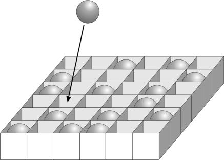
Figure 1: Sketch of the box model. Balls are thrown at random until all the cells of the box are full. Then the box is emptied and a new cycle starts.

The box represents the area of the fault or fault segment, and the random throwing of balls represents the increase of regional stress. This randomness is a way of dealing with the complex stress increase on actual faults. The occupation of a cell by a ball stands for the elastic strain induced by the stress in a patch or element of the fault plane. The loss of the balls that land on already occupied cells mimics stress dissipation on this plane. The total elastic strain (or conversely the total potential elastic energy) accumulated in the fault is represented by the number of occupied cells. This number gradually grows up to the limit $N$ (analogous to the failure threshold of the fault), and the toppling of the box represents the occurrence of the characteristic earthquake in the fault. It is easy to simulate the evolution of this system with a Monte Carlo approach.

This model is similar to that introduced by Newman and Turcotte in Ref. Newman478, . The difference is that their model is a square grid of cells in which the topology is relevant: they consider that the characteristic earthquake occurs when a percolating clusterStauffer spans the grid. This cluster happens before the grid is completely full.

III.2 Some formulas of the box model

To describe the box model analytically, it is convenient to recall some elements of the geometric distribution. Consider the probability that exactly $x$ independent Bernoulli trials, each with a probability of success $p$, will be required until the first success is achieved. The probability that $(x-1)$ failures will be followed by a success is $(1-p)^{x-1}p$. The resulting probability function,

$$f(x;p)=(1-p)^{x-1}p,$$ (4)

is known as the geometric distribution. Its mean and variance are

$$\langle x\rangle=\frac{1}{p},\qquad\sigma^{2}=\frac{1-p}{p^{2}}.$$ (5)

Now we deal with the box model further. In each cycle, the filling of the box proceeds sequentially and continues until the $N$th cell is occupied. Because each of these sequential steps is an independent process, the mean number of throws to completely fill the box will be

$$\langle n\rangle_{N}=\langle x_{1}\rangle_{N}+\langle x_{2}\rangle_{N}+\dots+\langle x_{N}\rangle_{N},$$ (6)

where $\langle x_{i}\rangle_{N}$ is the mean number of throws it takes to fill the ith cell.

Because the filling of the ith cell is geometrically distributed with $p_{i}=(N+1-i)/N$, it follows that

$$\langle x_{i}\rangle_{N}=\frac{N}{N+1-i},\qquad(i=1,2,\dots,N)$$ (7)

and therefore

$$\langle n\rangle_{N}=1+\sum_{i=2}^{N}\frac{N}{N+1-i}.$$ (8)

Relations similar to Eqs. (6) and (8) can be written for the variance of the number of thrown balls to fill the box, namely

$$\sigma_{N}^{2}=\sigma_{1}^{2}+\sigma_{2}^{2}+\dots=0+\sum_{i=2}^{N}\frac{1-\displaystyle\frac{N+1-i}{N}}{\left(\displaystyle\frac{N+1-i}{N}\right)^{2}},$$ (9)

and consequently, the standard deviation is

$$\sigma_{N}=\left[\sum_{i=2}^{N}\frac{N(i-1)}{(N+1-i)^{2}}\right]^{1/2}.$$ (10)

The aperiodicity of the series, $\alpha_{N}$, for a given $N$ is

$$\alpha_{N}=\frac{\sigma_{N}}{\langle n\rangle_{N}}.$$ (11)

The mean and the standard deviation of the box model can be calculated by summing the $N-1$ terms of Eqs. (8) and (10). For $N\geq 10$, these two equations can be approximated (with an absolute error $<0.01$) by their asymptotic expressions:asymptotic

$$\langle n\rangle_{N}\xrightarrow[N\to\infty]{}N(C+\ln N)+\frac{1}{2},$$ (12)

where $C\simeq 0.5772157$ is Euler’s constant, and

$$\sigma_{N}\xrightarrow[N\to\infty]{}N\left[\frac{\pi^{2}}{6}-\frac{1+C+\ln N}{N}\right]^{1/2},$$ (13)

and the aperiodicity can be estimated by using Eq. (11) with Eqs. (12) and (13).

The function $P_{N}(n)$ is not as easy to obtain as its mean and standard deviation, and is given by

$$P_{N}(n)=\sum_{j=1}^{N-1}(-1)^{j+1}{N-1\choose j-1}\Big{(}1-\frac{j}{N}\Big{)}^{n-1},$$ (14)

and the accumulative probability function, $A_{N}(n)$:

$$A_{N}(n) = \sum_{j=N}^{n}P_{N}(j)=$$

$$= 1-\sum_{j=1}^{N-1}(-1)^{j+1}{N-1\choose j-1}\Big{(}1-\frac{j}{N}\Big{)}^{n}\ \frac{N}{j}.$$

We have deduced Eq. (14) by means of a Markov chain approach analogous to the one used in Refs. VazquezPrada250, and Vazquez2, . This derivation is omitted here because of its length.

IV Fitting the parameters of the box model

We will fit the Parkfield series to the accumulative probability function, Eq. (III.2), using the method of moments.Utsu497 Another method that could be used is that of maximum likelihood.Utsu497 We have seen in Sec. III that the aperiodicity in the box model depends only on $N$. Thus, we will choose $N$ for which the aperiodicity is the closest to that of the Parkfield series, that is, $\alpha\simeq 0.3759$. The result is $N=11$, for which, from Eq. (11), the aperiodicity is $\alpha=0.3752$.

From Eq. (8) the mean value of $n$ for $N=11$ is $\langle n\rangle_{N=11}=33.22$. Because the actual mean of the Parkfield series is $m=24.62$ yr, one ball throw in the model is equivalent to $\tau=24.62\,\mbox{yr}/33.22=0.74\,\mbox{yr}\approx 9$ months. The discrete distribution function for the duration of the seismic cycle in a box model with $N=11$, $P_{11}(n)$ is shown in Fig. 2.

Figure 2: Discrete distribution function for the duration (in time steps, $n$) of the seismic cycle in the box model with $N=11$.

In Fig. 3 we plot the evolution of the number of occupied cells for ten cycles with $N=11$. Note the fluctuations in the duration of the cycles, which are consistent with the mean and the standard deviation of the series. Note also that the occupation increases rapidly just after a toppling, and then slows down. This increase is due to the fact that, as a cycle progresses, there are more occupied cells, and thus it is less probable for an incoming ball to land on an empty cell. If $\rho_{n}$ is the fraction of occupied cells at time step $n$, there is a probability $1-\rho_{n}$ for the next ball to be thrown to an empty cell. Because such a throw would increase $\rho$ by $1/N$, the mean $\rho$ at step $n+1$ is

$$\langle\rho_{n+1}\rangle=\langle\rho_{n}\rangle+\frac{1}{N}[1-\langle\rho_{n}\rangle].$$ (16)

The box is empty at the beginning of the cycle ($\rho_{0}=0$), so from Eq. (16), the mean value of $\rho_{n}$ is

$$\langle\rho_{n}\rangle=1-\Big{(}1-\frac{1}{N}\Big{)}^{n},$$ (17)

which approaches one asymptotically.

In real faults, the strain also does not increase uniformly during the seismic cycle. Instead, it follows a trend similar to that of the number of occupied cells in the box model: the loading rate is faster just after a large earthquake, and decreases over time.Michael548

The relaxation of a real fault by means of a large earthquake reduces the stress in the system. Thus a minimum time has to elapse before the fault accumulates enough stress to produce the next large earthquake. This effect is called stress shadow.Harris366 In the box model there exists a stress shadow: a characteristic earthquake cannot occur until the $N$th step in the cycle. According to the box model, this minimum time for the Parkfield series is $\tau N\simeq 8$ yr.

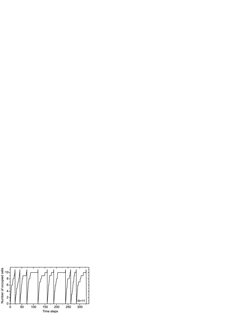
Figure 3: Plot of the number of occupied cells during ten cycles of a box model with $N=11$.

V Earthquake probabilities at Parkfield

We now evaluate the quality of the box model fit for the Parkfield series and estimate the probability of the next earthquake in this fault segment. In Fig. 4(a), the empirical distribution function of the Parkfield series is plotted. It is an accumulative step function ranging from 0 to 1.0, with a jump 1/6 at each of the six observed recurrence intervals $c_{i}$. The accumulated distribution of the box model in Eq. (III.2) for $N=11$ with $\tau=0.74$ yr also is drawn. In Fig. 4(b), we show the residuals of the fit, which do not surpass 7.5%. The equivalent fits to these data, made by using the renewal models cited in Sec. I, give very similar results.Gonzalez

Figure 4: (a) Fit of the accumulative distribution of the box model to the accumulated histogram of the Parkfield earthquake sequence. (b) Residuals of the fit, evaluated at the midpoints of the horizontal segments of the accumulated histogram.

Now we calculate the yearly probability of the next earthquake, that is, the conditional probability of the next shock occurring in a certain year, given that it has not occurred previously. For the box model it is

$$P_{\tau}(N,n)=\frac{A_{N}(n+1/\tau)-A_{N}(n)}{1-A_{N}(n-1)}.$$ (18)

Note that $1/\tau$ is the number of time steps of the box model corresponding to one year. After calculating $P_{\tau}$ from Eq. (18), it is necessary to rescale the abscissas, $n$, to actual years, $n\tau+t_{0}$, where $t_{0}$ is the calendar year at which the last earthquake occurred ($t_{0}=2004.75$ for the Parkfield series). In Fig. 5 we plot the yearly probability for the new cycle at Parkfield according to the box model. During the first eight years after the last earthquake at Parkfield (which occurred in September 2004), the box model indicates that another big shock should not be expected. From that time on, the probability of the next earthquake increases, tending to a constant equal to 11%.

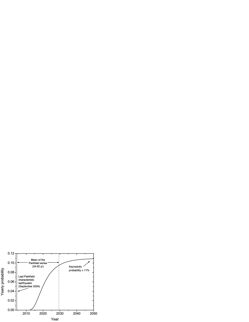
Figure 5: Yearly probability of the next characteristic earthquake at Parkfield, according to the box model.

In the seismological literature there is a well-known question about the yearly probability for a time much longer than the mean value of the series:Davis “The longer it has been since the last earthquake, the longer the expected time till the next?” Sornette and KnopoffSornette have discussed some statistical distributions that lead to affirmative, negative, or neutral answers to it. The result shown in Fig. 5 leads us to conclude that the box model produces a neutral answer. The reason is that for a long cycle duration (large $n$), the $P_{N}(n)$ of the box model decays exponentially, and asymptotically the box model behaves as a Poisson model, in which the conditional probability of occurrence of the next earthquake is a constant.

VI A Simple Forecasting Strategy

In earthquake forecasting an “alarm” is sometimes turned on when it is estimated that there is a high probability for a large earthquake to occur.KeilisBL If a large shock takes place when the alarm is on, the prediction is considered to be a success. If it takes place when the alarm is off, there has been a failure to predict. The fraction of errors, $f_{e}$, is the number of prediction failures divided by the total number of large earthquakes. The fraction of alarm time, $f_{a}$, is the ratio of the time during which the alarm is on to the total time of observation. A good strategy of forecasting must produce both small $f_{e}$ and $f_{a}$, because both the prediction failures and the alarms are costly. Depending on the trade-off between the costs and benefits of forecasting,Molchan2 we can try to minimize a certain loss function, $L$. For simplicity, we will consider a simple loss function defined as

$$L=f_{a}+f_{e}.$$ (19)

A random guessing strategy (randomly turning the alarm on and off) will yield $L=1$, a result which can be easily understood. The alarm will be on, randomly, during a certain fraction of time, $f_{a}$. Thus, there will be a probability equal to $f_{a}$ for it being on when an earthquake eventually occurs (and a probability of $1-f_{a}$ for it being off). The result is that $f_{e}=1-f_{a}$. As a trivial special case, if the alarm is always on ($f_{a}=1$), then all the earthquakes are “forecasted” ($f_{e}=0$). Conversely, all the earthquakes are failures to predict if the alarm is always off. The random guessing strategy is considered as a baseline, so a forecasting procedure makes sense only if it gives $f_{a}+f_{e}<1$.

We can use the box model fit to the Parkfield series to implement a simple earthquake forecasting strategy. The strategy consists in turning on the alarm at a fixed value of $n$ time steps after the last big earthquake, and maintaining the alarm on until the next one.Newman478 ; Vazquez2 Then the alarm is turned off, and the same strategy is repeated, evaluating $f_{a}$ and $f_{e}$ for all the cycles. The result is

$$f_{e}(n)=\sum_{n^{\prime}=1}^{n}P(n^{\prime}),$$ (20)

and

$$f_{a}(n)=\frac{\sum_{n^{\prime}=n}^{\infty}P(n^{\prime})(n^{\prime}-n)}{\sum_{n^{\prime}=0}^{\infty}P(n^{\prime})n^{\prime}}.$$ (21)

These relations are illustrated in Fig. 6(a), together with $L=f_{a}+f_{e}$. For each value of $N$, $L(n)$ has a minimum at a specific value of $n$, $n^{*}(N)$. As can be seen in Fig. 6(a), $n^{*}(11)=20$, for which

$$f_{a}(n^{*})=0.405,\quad f_{e}(n^{*})=0.085,\quad L(n^{*})=0.490.$$ (22)

For the Parkfield sequence, $n^{*}$ corresponds to

$$\tau n^{*}=14.8\,\mbox{yr}.$$ (23)

If the distribution derived from the box model correctly describes the recurrence of large earthquakes at Parkfield, the alarm connected at this time since the beginning of the cycles and disconnected just after the occurrence of each shock would yield the results given in Eq. (22). Note that this time is substantially smaller than the mean duration of the cycles, $m=24.62$ yr.

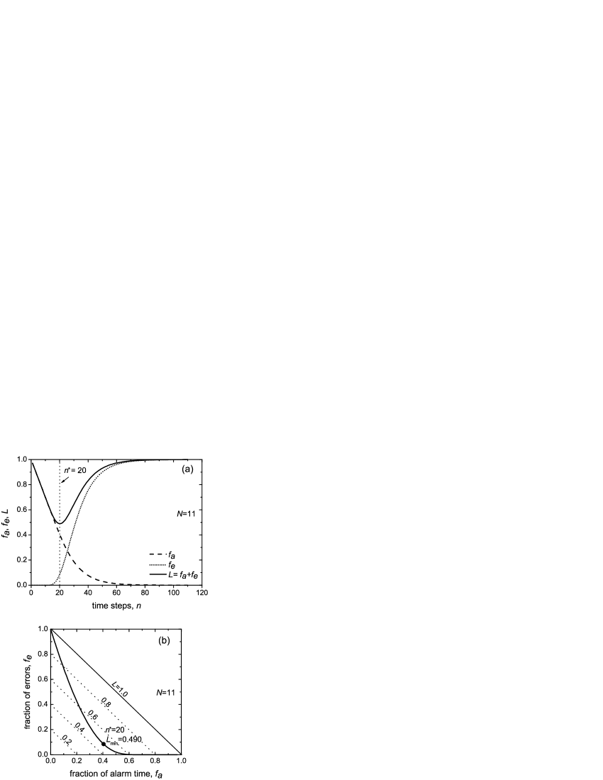
Figure 6: (a) Fraction of errors ($f_{e}$), fraction of alarm time ($f_{a}$), and loss function ($L=f_{a}+f_{e}$) as a function of $n$ for the forecasting strategy in a box model with $N=11$. (b) Error diagram for this strategy. Each point on the curve is the result of using a different value of $n$. The large dot corresponds to $n^{*}$, for which the loss function reaches a minimum. The diagonal lines are isolines of $L$. A random guessing strategy would render $L=1$.

The quality of the model-earthquake forecast also can be understood visually by means of an error diagram, Fig. 6(b), in which $f_{e}$ is plotted versus $f_{a}$.Molchan2 This kind of plot is similar to the receiver operating characteristic diagram, used, for example, to test the success of weather forecasts.Joliffe

VII Summary

The generation of large earthquakes in a seismic fault involves slow loading of elastic strain (or, conversely, elastic energy), and release through rupture and/or frictional sliding during an earthquake. The duration of this process is the seismic cycle, which is repeated indefinitely, leading to a series of recurrent shocks. We have illustrated this process with a very simple model. The loading of elastic strain is represented by the stochastic filling of a box with $N$ cells. The emptying of the box after its complete filling is analogous to the generation of a large earthquake, in which the fault relaxes after having being loaded to its failure threshold. The duration of the filling process is thus equivalent to the seismic cycle.

The statistical distribution of seismic cycles in the box model (just as the distributions of the Brownian passage time modelMatthews and the minimalist modelVazquezPrada250 ; Vazquez2 ; Gomez&Pacheco546 ) can be used to fit actual earthquake series and to estimate earthquake probabilities. The conditional probability of the box model has two interesting features. First, after a large earthquake, there is a period of stress shadow during which a new large earthquake cannot occur. Second, from this time on the probability continuously increases, approaching a constant asymptotic value. By using a simple forecasting strategy, we have shown that the earthquakes in the model are predictable to some extent.

We hope that our discussion will be a useful educational tool for introducing several important geophysical and statistical concepts to graduate and undergraduate students. It could illustrate how to make quantitative estimates of a natural phenomenon as popular and as mystifying as earthquakes.

- (1) Harry Fielding Reid, “The mechanics of the earthquake,” in The California earthquake of April 18, 1906, Report of the State Earthquake Investigation Comission (Carnegie Institution, Washington, DC, 1910), Vol. 2, pp. 1–192.
- (2) Robert S. Yeats, Kerry Sieh, and Clarence R. Allen, The Geology of Earthquakes (Oxford University Press, New York, 1997).
- (3) Grove Karl Gilbert, “A theory of the earthquakes of the Great Basin, with a practical application,” Am. J. Sci. Ser. 3, 27(157), 49–54 (1884).
- (4) Grove Karl Gilbert, “Earthquake forecasts,” Science XXIX(734), 121–138 (1909).
- (5) Alexander McKay, “On the earthquakes of September 1888, in the Amuri District,” N. Z. Geol. Surv. Rep. Geol. Explor. 1888–1889, 20, 1–16 (1890).
- (6) Bunjiro Koto, “On the cause of the great earthquake in central Japan, 1891,” J. Coll. Sci. Imp. Univ. Tokyo 5, 296–353 (1893).
- (7) David P. Schwartz and Kevin J. Coppersmith, “Fault behavior and characteristic earthquakes: Examples from the Wasatch and San Andreas fault zones,” J. Geophys. Res. 89(B7), 5681–5698 (1984).
- (8) GeoComplexity and the Physics of Earthquakes, edited by John B. Rundle, Donald L. Turcotte, and William Klein (American Geophysical Union, Washington, DC, 2000).
- (9) Eric Bonnet, Olivier Bour, Noelle E. Odling, Philippe Davy, Ian Main, Patience Cowie, and Brian Berkowitz, “Scaling of fracture systems in geological media,” Rev. Geophys. 39(3), 347–383 (2001).
- (10) Ruth A. Harris, “Earthquake stress triggers, stress shadows, and seismic hazard,” Curr. Sci. 79(9), 1215–1225 (2000).
- (11) James C. Savage, “Empirical earthquake probabilities from observed recurrence intervals,” Bull. Seismol. Soc. Am. 84(1), 219–221 (1994).
- (12) David Vere-Jones, “Stochastic models for earthquake occurrence (with discussion),” J. R. Statis. Soc. Ser. B. Metodol. 32, 1–62 (1970).
- (13) Tokuji Utsu, “Large earthquakes near Hokkaido and the expectancy of the occurrence of a large earthquake of Nemuro,” Rep. Coord. Comm. Earthq. Predict. 7, 7–13 (1972).
- (14) Tokuji Utsu, “Aftershocks and earthquake statistics (IV),” J. Fac. Sci. Hokkaido Univ. Ser. VII 4, 1–42 (1972).
- (15) Tsuneji Rikitake, “Probability of earthquake occurrence as estimated from crustal strain,” Tectonophysics 23(3), 299–312 (1974).
- (16) Yukio Hagiwara, “Probability of earthquake occurrence as obtained from a Weibull distribution analysis of crustal strain,” Tectonophysics 23(3), 313–318 (1974).
- (17) Tsuneji Rikitake, “Recurrence of great earthquakes at subduction zones,” Tectonophysics 35(4), 335–362 (1976).
- (18) David Vere-Jones, “Earthquake prediction: A statistician’s view,” J. Phys. Earth 26, 129–146 (1978).
- (19) Erhan Çinlar, Introduction to Stochastic Processes (Prentice Hall, New York, 1975).
- (20) Daryl J. Daley and David Vere-Jones, An Introduction to the Theory of Point Processes (Springer-Verlag, New York, 2003), 2nd ed.
- (21) Tokuji Utsu, “Estimation of parameters for recurrence models of earthquakes,” Bull. Earthquake Res. Inst. Univ. Tokyo 59, 53–66 (1984).
- (22) Stuart P. Nishenko and Raymond Buland, “A generic recurrence interval distribution for earthquake forecasting,” Bull. Seismol. Soc. Am. 77(4), 1382–1399 (1987).
- (23) Anne S. Kiremidjian and Thalia Anagnos, “Stochastic slip-predictable model for earthquake occurrences,” Bull. Seismol. Soc. Am. 74(2), 739–755 (1984).
- (24) Kerry Sieh, Minze Stuiver, and David Brillinger, “A more precise chronology of earthquakes produced by the San Andreas fault in southern California,” J. Geophys. Res. 94(B1), 603–623 (1989).
- (25) Nancy R. Mann, Ray E. Schafer, and Nozer D. Singpurwalla, Methods for Statistical Analysis of Reliability and Life Data (John Wiley and Sons, New York, 1974).
- (26) Ian Main, “Statistical physics, seismogenesis, and seismic hazard,” Rev. Geophys. 34(4), 433–462 (1996).
- (27) Yehuda Ben-Zion, “Dynamic ruptures in recent models of earthquake faults,” J. Mech. Phys. Solids 49(9), 2209–2244 (2001).
- (28) Steven N. Ward, “San Francisco Bay area earthquake simulations: A step toward a standard physical earthquake model,” Bull. Seismol. Soc. Am. 90(2), 370–386 (2000).
- (29) Russell Robinson, “Potential earthquake triggering in a complex fault network: the northern South Island, New Zealand,” Geophys. J. Int. 159(2), 734-748 (2004).
- (30) Mark V. Matthews, William L. Ellsworth, and Paul A. Reasenberg, “A Brownian model for recurrent earthquakes,” Bull. Seismol. Soc. Am. 92(6), 2233–2250 (2002).
- (31) Miguel Vázquez-Prada, Álvaro González, Javier B. Gómez, and Amalio F. Pacheco, “A minimalist model of characteristic earthquakes,” Nonlinear Processes Geophys. 9(5-6), 513–519 (2002).
- (32) Miguel Vázquez-Prada, Álvaro González, Javier B. Gómez, and Amalio F. Pacheco, “Forecasting characteristic earthquakes in a minimalist model,” Nonlinear Processes Geophys. 10(6), 565–571 (2003).
- (33) Javier B. Gómez and Amalio F. Pacheco, “The minimalist model of characteristic earthquakes as a useful tool for description of the recurrence of large earthquakes,” Bull. Seismol. Soc. Am. 95(5), 1960–1967 (2004).
- (34) Álvaro González, Javier B. Gómez, and Amalio F. Pacheco, “Updating seismic hazard at Parkfield,” J. Seismol., in press, physics/0411003.
- (35) Masajiro Imoto, “Probability gains expected for renewal process models,” Earth, Planets Space 56(6), 563–571 (2004).
- (36) Working Group on California Earthquake Probabilities, “Earthquake probabilities in the San Francisco Bay Region: 2002–2031,” Open-File Report 03-214 (United States Geological Survey, Menlo Park, CA, 2003).
- (37) William H. Bakun and Allan G. Lindh, “The Parkfield, California, earthquake prediction experiment,” Science 229, 619–624 (1985).
- (38) Evelyn Roeloffs, “The Parkfield, California earthquake experiment: An update in 2000,” Curr. Sci. 79(9), 1226–1236 (2000).
- (39) William H. Bakun, “History of significant earthquakes in the Parkfield area,” Earthq. Volcano. 20(2), 45–51 (1988).
- (40) Bruce D. Malamud and Donald L. Turcotte, “Cellular-automata models applied to natural hazards,” Comput. Sci. Eng. 2(3), 42–51 (2000).
- (41) Zeev Olami, Hans Jacob S. Feder, and Kim Christensen, “Self-organized criticality in a continuous, nonconservative cellular automaton modeling earthquakes,” Phys. Rev. Lett. 68(8), 1244–1247 (1992).
- (42) Eric F. Preston, Jorge S. Sá Martins, John B. Rundle, Marian Anghel, and William Klein, “Models of earthquake faults with long-range stress transfer,” Comput. Sci. Eng. 2(3), 34–41 (2000).
- (43) Stephen A. Miller, “Properties of large ruptures and the dynamical influence of fluids on earthquakes and faulting,” J. Geophys. Res. 107, 2182 (2002).
- (44) William I. Newman and Donald L. Turcotte, “A simple model for the earthquake cycle combining self-organized complexity with critical point behavior,” Nonlinear Processes Geophys. 9(5-6), 453–461 (2002).
- (45) Dietrich Stauffer and Amnon Aharony, Introduction to Percolation Theory (Taylor and Francis, London, 1994), 2nd ed.
- (46) I. S. Gradshteyn and I. M. Ryzhik, Table of Integrals, Series, and Products (Academic Press, New York, 1965).
- (47) Andrew J. Michael, “Viscoelasticity, postseismic slip, fault interactions, and the recurrence of large earthquakes,” EOS Trans. Am. Geophys. Union 84(46), Fall. Meet. Suppl., Abstract S31G-04 (2003). The paper corresponding to this abstract has been submitted to Bull. Seismol. Soc. Am.
- (48) Paul M. Davis, David D. Jackson, and Yan Y. Kagan, “The longer it has been since the last earthquake, the longer the expected time till the next?,” Bull. Seismol. Soc. Am. 79(5), 1439–1456 (1989).
- (49) Didier Sornette and Leon Knopoff, “The paradox of the expected time until the next earthquake,” Bull. Seismol. Soc. Am. 87(4), 789–798 (1997).
- (50) Nonlinear Dynamics of the Lithosphere and Earthquake Prediction, edited by Vladimir I. Keilis-Borok and Alexandre A. Soloviev (Springer-Verlag, Berlin, Germany, 2003).
- (51) George M. Molchan, “Earthquake prediction as a decision-making problem,” Pure Appl. Geophys. 149(1), 233–247 (1997).
- (52) Ian B. Mason, “Binary forecasts,” in Forecast Verification: A Practitione’s Guide in Atmospheric Science, edited by Ian T. Joliffe and David B. Stephenson (Wiley, West Sussex, UK, 2003), pp. 37-76 (references on pp. 215-226).