Detailed analysis of a pseudoresonant interaction between cellular flames and velocity turbulence

Abstract

This work is dedicated to the analysis of the delicate details of the effect of upstream velocity fluctuations on the flame propagation speed. The investigation was carried out using the Sivashinsky model of cellularisation of hydrodynamically unstable flame fronts. We identified the perturbations of the steadily propagating flames which can be significantly amplified over finite periods of time. These perturbations were used to model the effect of upstream velocity fluctuations on the flame front dynamics and to study a possibility to control the flame propagation speed.

Key words: hydrodynamic flame instability, Sivashinsky equation, nonmodal amplification, flame-turbulence interaction

AMS subject classification: 35S10, 76E17, 80A25, 65F15

Abbreviated title: Analysis of pseudoresonant flame-turbulence interaction

1 Introduction

Experiments show that cellularisation of flames results in an increase of their propagation speed. In order to understand and exploit this phenomenon, we study the evolution of flame fronts governed by the Sivashinsky equation

$$\partial_{t}\Phi-2^{-1}\left(\partial_{x}\Phi\right)^{2}=\partial_{xx}\Phi-(\gamma/2)\partial_{x}\mathcal{H}[\Phi]+f(x,t),\qquad-\infty<x<\infty,\quad t>0$$ (1)

with the force term $f(x,t)$. Here $\Phi(x,t)$ is the perturbation of the plane flame front, $\mathcal{H}[\Phi]=\pi^{-1}\int_{-\infty}^{\infty}(x-\xi)^{-1}\Phi(\xi,t)d\xi$ is the Hilbert transformation, and $\gamma=1-\rho_{b}/\rho_{u}$ is the contrast in densities of burnt and unburnt gases $\rho_{b}$ and $\rho_{u}$ respectively. Initial perturbation $\Phi(x,0)$ is given.

The equation without the force term was obtained in [1] as an asymptotic mathematical model of cellularisation of flames subject to the hydrodynamic flame instability. The force term was suggested in [2] in order to account for the effect of the upstream turbulence on the flame front. It is equal to the properly scaled turbulent fluctuations of the velocity field of the unburned gas. In [3] and [4] equation (1) was further refined in order to include effects of the second order in $\gamma$. However, as mentioned in [4], this modification can be compensated upon a Galilean transformation combined with a nonsingular scaling. Thus, we have chosen to remain within the first order of accuracy in $\gamma$ of the original Sivashinsky model (1) as it should have the same qualitative properties as the more quantitatively accurate one.

The asymptotically stable solutions to the Sivashinsky equation with $f(x,t)\equiv 0$ corresponding to the steadily propagating cellular flames do exist and are given by formula

$$\Phi_{N,L}(x,t)=V_{N,L}t+2\sum\limits_{n=1}^{N}\ln|\cosh 2\pi b_{n}/L-\cos 2\pi x/L|,$$ (2)

discovered in [5]. Here, real $L>0$ and integer $N$ from within the range $0\leq N\leq N_{L}=\operatorname*{ceil}(\gamma L/8\pi+1/2)-1$ are otherwise arbitrary parameters. Also, $V_{L}=2\pi NL^{-1}\left(\gamma-4\pi NL^{-1}\right)$, and $b_{1},b_{2},\ldots,b_{N}$ satisfy a system of nonlinear algebraic equations available elsewhere. Functions (2) have a distinctive set of $N$ complex conjugate pairs of poles $z_{n}=\pm ib_{n}$, $n=1,\ldots,N$ and are called the steady coalescent pole solutions respectively.

The steady coalescent pole solutions (2) with the maximum possible number $N=N_{L}$ of the poles were found to be asymptotically, for $t\rightarrow\infty$, stable if the wavelength of the perturbations does not exceed $L$, see [6]. However, in spite of their asymptotic stability, there are perturbations of these solutions which can be hugely amplified over finite intervals of time resulting in significant transients, see [7]. These perturbations are nonmodal, because they cannot be represented by the single eigenmodes of the linearised Sivashinsky equation. In what follows we are interested in solutions (2) with $N=N_{L}$ and retain the index $L$ only. Also, in all reported calculations $\gamma=0.8$.

In this work we calculate the most amplifiable nonmodal perturbations to the asymptotically stable cellular solutions of the Sivashinsky equation and use them to investigate the response of the flame front to forcing. In particular, we study the effect of stochastic forcing or noise. The investigation of the effect of noise in the Sivashinsky equation was carried out numerically and the observations were reinforced by the analytical analysis of an approximation to the linearised Sivashinsky equation suggested in [8].

2 The largest growing perturbations

Substituting $\Phi(x,t)=\Phi_{L}(x,t)+\phi(x,t)$ into (1) for $f(x,t)\equiv 0$ and linearising it with respect to the $L$-periodic perturbations $\phi(x,t)$, one obtains

$$\left\{\begin{array}[]{l}\partial_{t}\phi=(\partial_{x}\Phi_{L})\partial_{x}\phi+\partial_{xx}\phi-(\gamma/2)\partial_{x}{\cal H}[\phi]=A_{L}\phi,\\ \\ \phi(x,0)=\Phi(x,0)-\Phi_{L}(x,0).\end{array}\right.$$ (3)

The operator $A_{L}$ generates the evolution operator $e^{tA_{L}}$, which provides the solution to (3) in the form $\phi(x,t)=e^{tA_{L}}\phi(x,0)$.

Assuming that the polar decomposition of the evolution operator does exist, we write it as

$$e^{tA_{L}}=\mathcal{U}(t)\mathcal{S}(t),$$ (4)

where $\mathcal{U}(t)$ is a partially isometric and $\mathcal{S}(t)=\left[\left(e^{tA_{L}}\right)^{*}e^{tA_{L}}\right]^{1/2}$ is the nonnegative self-adjoint operator, see e.g. [9]. The partial isometry of $\mathcal{U}(t)$ implies that it preserves the norm when mapping between the sets of values of $\left(e^{tA_{L}}\right)^{*}$ and $e^{tA_{L}}$, i.e. $\|\mathcal{U}(t)\phi\|=\|\phi\|$. Then, under certain conditions, $\|\phi(x,t)\|=\|\mathcal{S}(t)\phi(x,0)\|$ and for the $2$-norm the $\sup\limits_{\phi(x,0)\in\mathcal{D}\left(e^{tA_{L}}\right)}\left\{\|\mathcal{S}(t)\phi(x,0)\|\right.$ $\left.\times\|\phi(x,0)\|^{-1}\right\}$ is equal to the largest eigenvalue $\sigma_{1}(t)$ of $\mathcal{S}(t)$. This eigenvalue is associated with the eigenvector $\psi_{1}(x,t)$ of $\mathcal{S}(t)$.

The eigenvectors $\psi_{\alpha}(x,t)$ of $\mathcal{S}(t)$ are mutually orthogonal at any given time $t=t^{*}$ and can be used as a basis in the space of the admissible initial conditions $\phi(x,0)$ $=\sum\limits_{\alpha=1}^{\infty}c_{\alpha}(0,t^{*})$ $\times\psi_{\alpha}(x,t^{*})$. Then, the associated eigenvalues $\sigma_{\alpha}(t^{*})$ provide the magnitudes of amplification of the $\psi_{\alpha}(x,t^{*})$ components of the initial condition $\phi(x,0)$ by the time instance $t^{*}$. Note, that for (3) the $2$-norm of the perturbation $\phi(x,t)$ is just its energy and that the eigenvalues $\sigma_{\alpha}(t)$, $\alpha=1,2,\ldots$ and eigenvectors $\psi_{\alpha}(x,t)$ of $\mathcal{S}(t)$ are the singular values and the right singular vectors of $e^{tA_{L}}$ respectively.

According to [10], the Fourier image $\widetilde{A_{L}}$ of the operator $A_{L}$ is defined by the $(k,l)$-th entry of its double infinite ($-\infty<k,l<\infty$) matrix

$$(\widetilde{A_{L}})_{k,l}=\left(-\frac{4\pi^{2}}{L^{2}}k^{2}+\frac{\pi\gamma}{L}|k|\right)\delta_{k,l}+\frac{8\pi^{2}}{L^{2}}l\operatorname*{sign}(k-l)\sum\limits_{n=1}^{N_{L}}e^{-2\pi b_{n}|k-l|/L},$$ (5)

where $\delta_{k,l}$ is the Kronecker’s symbol. By limiting our consideration to the first $K$ harmonics, we approximate our double infinite matrix $\widetilde{A_{L}}$ with the $(2K+1)\times(2K+1)$ matrix $\widetilde{A_{L}^{(K)}}$, whose entries coincide with those of $\widetilde{A_{L}}$ for $-K\leq k,l\leq K$. Then, the matrix $e^{t\widetilde{A_{L}^{(K)}}}\approx\widetilde{e^{tA_{L}}}$ can be effectively evaluated by the scaling and squaring algorithm with a Padé approximation. Eventually, the required estimations of $\sigma_{\alpha}(t)$ and Fourier images of $\psi_{\alpha}(x,t)$ can be obtained through the singular value decomposition (SVD) of $e^{t\widetilde{A_{L}^{(K)}}}$, see e.g. [11].

Indeed, if the SVD of $e^{t\widetilde{A_{L}^{(K)}}}$ is given by

$$e^{t\widetilde{A_{L}}^{(K)}}=\mathcal{W}(t)\mathcal{D}(t)\mathcal{V}(t)^{*},$$ (6)

where $\mathcal{W}(t)$, $\mathcal{V}(t)$ are unitary and $\mathcal{D}(t)$ is the nonnegative diagonal matrix, then the matrices

$$\mathcal{U}(t)=\mathcal{W}(t)\mathcal{V}(t)^{*},\qquad\mathcal{S}(t)=\mathcal{V}(t)\mathcal{D}(t)\mathcal{V}(t)^{*}$$ (7)

satisfy the adequate finite-dimensional projection of the polar decomposition (4) and the eigenvalues $\sigma_{\alpha}(t)$, $\alpha=1,2,\ldots$ and eigenvectors $\psi_{\alpha}(x,t)$ of $\mathcal{S}(t)$ are just the singular values and the Fourier syntheses of the right singular vectors of $e^{t\widetilde{\mathcal{A}_{L}}^{(K)}}$ respectively.

Graphs showing dependence of a few largest singular values of $e^{tA_{L}}$ versus time are shown in Fig. 1. One may see that values of $\sigma_{1,2}(t)$ for large enough $t$ match the estimation of the largest possible amplification of the perturbations $\phi(x,t)$ obtained in [7] by a different method. An even more impressive observation is that the dimension of the subspace of the significantly amplifiable perturbations is very low. Perturbations of only two types can be amplified by about $10^{6}$ times.

Figure 1: Twelve largest singular values of $e^{tA_{L}}$.

The initial conditions $\phi(x,0)$, which would be the most amplified once by $t^{*}=100$, $200$, $300$ and $10^{3}$, i.e. $\psi_{\alpha}(x,t^{*})$, are depicted in Fig. 2. The dominating singular modes $\psi_{\alpha}(x,t)$ stabilize to some limiting functions for $t>300$. For example, their graphs for $t=500$ and $t=10^{3}$ are indistinguishable in Fig. 2. However, they vary in time significantly when $t<300$ and for $t=200$ the associated amplification $\sigma_{1,2}(200)$ is already about $10^{3}$, though $\psi_{1,2}(x,200)$ does not coincide with neither $\psi_{1,2}(x,10^{3})$ nor $\psi_{3,4}(x,10^{3})$. Thus, the dependence of $\psi_{\alpha}$ on time makes the dimension of the subspace of perturbations, which can be amplified say about $10^{3}$ times much higher than two in contrast to what could be concluded from the graphs in Fig. 1. This illustrates the complicatedness of studies of the effect of transient amplification on short time scales $t<300$.

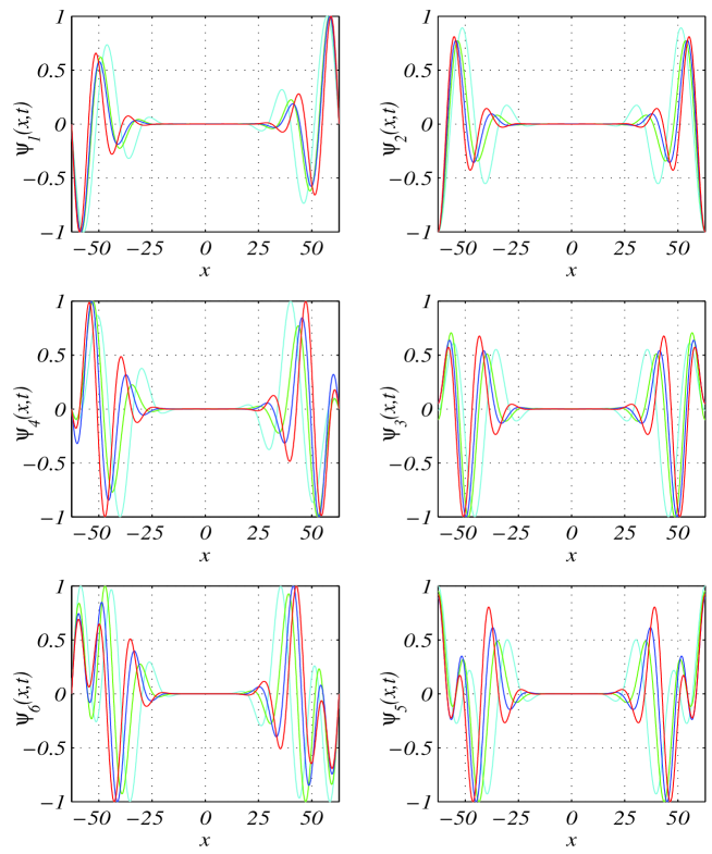
Figure 2: Right singular vectors of $e^{tA_{L}}$ corresponding to the six largest $\sigma_{\alpha}(t)$ for $t=100$ (cyan), $200$ (green), $300$ (blue), and $10^{3}$ (red).

Fourier components of $\psi_{1}(x,t^{*})$ and $\psi_{2}(x,t^{*})$ for $t^{*}=10^{3}$ are depicted in Fig. 3.

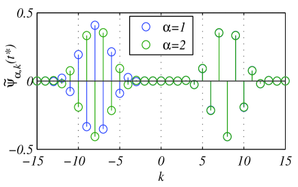
Figure 3: Fourier coefficients of $\psi_{\alpha}(x,t^{*})=\sum\limits_{k=-\infty}^{\infty}\widetilde{\psi}_{\alpha,k}(t^{*})e^{i2\pi kx/L}$ for $t^{*}=10^{3}$.

Evolution of the perturbations, which grow the most and is governed by the nonlinear Sivashinsky equation, is illustrated in Fig. 4. All the profiles were displaced vertically in order to compensate for steady propagation of flames in such a way that their spatial averages are equal to zero. Matching graphs of the spatially averaged flame propagation speed

$$<\Phi_{t}>=\frac{1}{L}\int\limits_{-L/2}^{L/2}\partial_{t}\Phi(x,t)dx,$$ (8)

are shown as well. The initial conditions were $\Phi(x,0)=\Phi_{L}(x,0)+\varepsilon\psi_{\alpha}(x,t^{*})$, where $\varepsilon=\pm 10^{-3}$, $\alpha=1,2$, and $t^{*}=10^{3}$. The computational method used in this work was presented in [12].

The asymmetric singular mode $\psi_{1}(x,t^{*})$ results in appearance of a small cusp to the left or to the right from the trough of $\Phi_{L}(x,0)$ depending on the sign of $\varepsilon$. After the cusp merges with the trough, the flame profile converges slowly to $\Phi_{L}(x+\Delta x,t)$, where $\operatorname*{sign}(\varepsilon)\Delta x>0$. For a positive $\varepsilon=10^{-3}$ the effect is illustrated in Fig. 4. Graphs of $\Phi(x,t)$ for $\varepsilon=-10^{-3}$ are exact mirror reflections of those depicted in 4(a) and graphs of $<\Phi_{t}>$ are exactly the same.

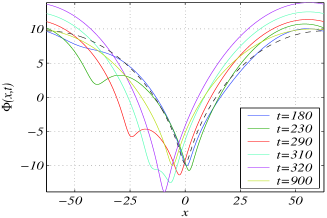
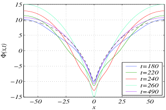
(a) $\varepsilon=10^{-3}$, $\alpha=1$		(b) $\varepsilon=-10^{-3}$, $\alpha=2$
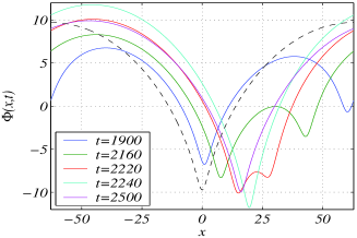
(c) $\varepsilon=10^{-3}$, $\alpha=2$		(d) $\varepsilon=10^{-3}$, $\alpha=2$, continues (c)

Figure 4: Solutions to (1) for $\Phi(x,0)=\Phi_{L}+\varepsilon\psi_{\alpha}(x,t^{*})$ and $L=40\pi$.

The symmetric singular mode $\psi_{2}(x,t^{*})$ produces two symmetric dents moving towards the trough on both sides of the profile if $\varepsilon<0$, see Fig. 4(b). By $t\approx 500$ the flame profile returns very closely to $\Phi_{L}(x,t)$. For $\varepsilon>0$ two small cusps move towards the boundaries of the computational domain creating a quasi-steady structure shown in Fig. 4(c) for $t=270$. This structure survives until $t\approx 1800$, but eventually bifurcates, see Fig. 4(d), and the solution converges to $\Phi_{L}(x+\Delta x,t)$, $\Delta x<0$. It looks like the bifurcation in question is associated with the lack of the asymptotic stability of the intermediate quasi-steady structure. As such, it was triggered by a random perturbation and could equally result in the displacement of the limiting flame front profile into the opposite direction $\Delta x>0$.

Behavior of perturbations $\psi_{1,2}(x,t^{*})$ of the amplitude $\varepsilon=10^{-6}$ was not as impressive, but they managed to produce a visible effect on the flame front profile. The same can be said about $\psi_{3,4}(x,t^{*})$ of the amplitude $\varepsilon=10^{-3}$. Perturbations corresponding to $\psi_{\alpha}(x,t^{*})$ of higher orders did not grow significantly and did not cause any noticeable changes to $\Phi_{L}$ for $\varepsilon$ up to $10^{-2}$.

Thus, the singular modes $\psi_{1,2}(x,t^{*})$ should be responsible for the interaction of the flame front $\Phi_{L}(x,t)$ with all the perturbations of small enough amplitude. The time scale of these interactions is about $300$ for $L=40\pi$ and is of order $O(L)$ in general. More singular modes $\psi_{\alpha}(x,t^{*})$ of higher orders $\alpha>2$ are becoming important as the amplitude of the perturbations grows. The time scale of evolution of $\phi(x,t)$ for $\phi(x,0)=\psi_{\alpha}(x,t^{*})$ lessens as $\alpha$ grows necessitating to take into account the dependence of $\psi_{\alpha}(x,t^{*})$ on $t^{*}$ and creating further problems in the efficient description of the subspace of important perturbations. Therefore, there is a critical perturbation amplitude beyond which the representation of $f(x,t)$ in terms of the singular modes $\psi_{\alpha}(x,t^{*})$ is not as beneficial as for smaller amplitudes.

3 A simplified linear model

Prior to experimenting with (1) we consider a simplified linear model suggested in [8]. The $L$-periodic steady coalescent $N_{L}$-pole solution (2) has a characteristic wavy or cellular structure and can be represented in a vicinity of the crest as $\Phi_{L}(x,t)\approx\Phi_{L}(0,t)-x^{2}/(2R)+O(x^{4})$. Here, $R$ is the radius of curvature of the flame front profile in the crest. For large enough $L$, it can be approximated as $R=c_{1}L+c_{2}$, where $c_{1}$ and $c_{2}$ are some constants. Note, that in the approximation of $\Phi_{L}(x,t)$ the origin $x=0$ was chosen exactly in the crest of $\Phi_{L}(x,t)$. Thus, $\partial_{x}\Phi_{L}\approx-x/R+O(x^{3})$ in a vicinity of $x=0$ and the equation suggested in [8] can be written as

$$\partial_{t}\phi+R^{-1}x\partial_{x}\phi=\partial_{xx}\phi+(\gamma/2)\partial_{x}\mathcal{H}[\phi]+f(x,t),$$ (9)

where $-\infty<x<\infty$ and $t>0$. The latter equation is much simpler than (3), yet it is meaningful enough to study the development of perturbations of $\Phi_{L}(x,t)$ appearing in the crest.

Equation (9) can be solved exactly. Applying the Fourier transformation we obtain

$$\partial_{t}\mathcal{F}[\phi]-R^{-1}\xi\partial_{\xi}\mathcal{F}[\phi]=-\left(4\pi^{2}\xi^{2}-\pi\gamma|\xi|-R^{-1}\right)\mathcal{F}[\phi]+\mathcal{F}[f](\xi,t),$$ (10)

which is a linear non-homogeneous hyperbolic equation of the first order. Using the standard method of characteristics its exact solution can be written as follows

$$\mathcal{F}[\phi](\xi,t)=\mathcal{G}(\xi,t)\mathcal{F}[\phi^{(0)}](|\xi|e^{t/R})+\int\limits_{0}^{t}\mathcal{G}(\xi,t-\tau)\mathcal{F}[f]\left[|\xi|e^{(t-\tau)/R},\tau\right]d\tau,$$ (11)

where

$$\mathcal{G}(\xi,t)=e^{t/R-2\pi^{2}R\left(e^{2t/R}-1\right)\xi^{2}+\pi\gamma R\left(e^{t/R}-1\right)|\xi|},$$ (12)

and $\mathcal{F}[f](\xi,t)=\int_{-\infty}^{\infty}f(x,t)e^{-i2\pi x\xi}dx$ denotes the Fourier transformation of $f(x,t)$.

If the initial condition is a single harmonics $\phi^{(0)}(x)=\cos(2\pi\xi_{0}x+\varphi)$ and $f(x,t)\equiv 0$, then

$$\phi(x,t)=e^{-2\pi^{2}R\left(1-e^{-2t/R}\right)\xi_{0}^{2}+\pi\gamma R\left(1-e^{-t/R}\right)\xi_{0}}\cos\left(2\pi\xi_{0}xe^{-t/R}+\varphi\right).$$ (13)

The infinite time limit of (13) is equal $e^{-2\pi^{2}R\xi_{0}^{2}+\pi\gamma R\xi_{0}}\cos\varphi$ and is reached effectively on the time scale of order $O(R)$. This time limit attains its maximum $e^{\gamma^{2}R/8}\cos\varphi$ for $\xi_{0}=\xi^{*}=\gamma/(4\pi)$, matching the asymptotic estimation of [8]. Note that the wave number of the largest Fourier component $k^{*}$ of both $\psi_{1}(x,t^{*})$ and $\psi_{2}(x,t^{*})$ for $t^{*}>300$ is equal to $\xi^{*}=k^{*}/L=\gamma/(4\pi)$ as well, see Fig. 3. A few graphical examples of function (13) are given in Fig. 5. Note that the argument of the cosine in (13) depends on time, which means that even if the initial condition $\phi^{(0)}(x)$ is a linear combination of mutually orthogonal cosine harmonics, then the solution $\phi(x,t)$ will remain a linear combination of cosine harmonics for $t>0$, but those harmonics will no longer be mutually orthogonal. This explains why the most amplified perturbations are formed by linear combinations of a few initially orthogonal harmonics and approximate $\psi_{1,2}(x,t^{*})$ asymptotically for $L\rightarrow\infty$.

(a) $\xi_{0}=\gamma/(2\pi)$, $\varphi=0$		(b) $\xi_{0}=\gamma/(4\pi)$, $\varphi=0$
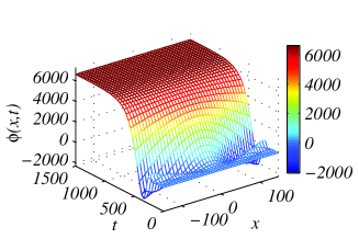
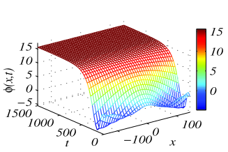
(c) $\xi_{0}=\gamma/(8\pi)$, $\varphi=0$		(d) $\xi_{0}=\gamma/(32\pi)$, $\varphi=0$
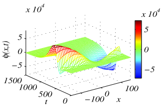
(e) $\xi_{0}=\gamma/(4\pi)$, $\varphi=\pi/4$		(f) $\xi_{0}=\gamma/(4\pi)$, $\varphi=\pi/2$

Figure 5: Examples of solutions (13) for $R=146.7126$, which corresponds to $L=40\pi$.

Behaviour of (13) is in a sharp contrast with the evolution of the single harmonics perturbations of the plane flame front

$$\phi(x,t)=e^{\left(-4\pi^{2}\xi_{0}^{2}+\pi\gamma\xi_{0}\right)t}\cos(2\pi\xi_{0}x+\varphi),$$ (14)

which grow infinitely if $\xi_{0}<\gamma/(4\pi)$ or decay otherwise. They are governed by the equation associated with a self-adjoint differential operator, which is obtained from (9) upon removal of the term $R^{-1}x\partial_{x}\phi$. Solution (14) does not result from (13) for $R\rightarrow\infty$, but is only equivalent to it when $t/R\ll 1$. The difference between (13) and (14) is an explicit illustration of the nonnormality of (9) introduced by the non-selfadjoint term $R^{-1}x\partial_{x}\phi$. Flattening of the crests of cellular flames and increasing local resemblance with the plane front as $R$ increases was noticed long time ago, prompting a hypothesis of a secondary Darrieus-Landau instability. Model (9) indicates that the hypothesis is unlikely to be correct. Although, because of the flattening of the crests of the flame front profile, perturbations of the front can be transiently amplified at a rate rapidly increasing with $R$, this transient amplification is entirely different from the infinite growth of perturbations in the Darrieus-Landau instability of plane flames. Moreover dynamics of perturbations in the case of cellular flames does not converge to that of the plane ones continuously in the limit $R\rightarrow\infty$.

Solution (11), (12) for $\phi(x,0)=e^{-px^{2}}$, $p>0$ can be represented in a closed form as well. Routine integration yields

$$\phi(x,t)=\frac{\pi}{\sqrt{pa}}e^{\frac{t}{R}+\frac{b^{2}-4\pi^{2}x^{2}}{4a}}\left\{\cos\frac{\pi bx}{a}+\Re\left[e^{\frac{i\pi bx}{a}}\operatorname*{erf}\left(\frac{b+i2\pi x}{2\sqrt{a}}\right)\right]\right\},$$ (15)

where

$$a=a(t)=2\pi^{2}R\left(e^{2t/R}-1\right)+\pi^{2}e^{2t/R}/p,\qquad b=b(t)=\pi\gamma R\left(e^{t/R}-1\right).$$ (16)

The result is illustrated in Fig. 6, where case (c) corresponds to the maximum growing perturbation of type $\phi(x,0)=e^{-px^{2}}$ and initial condition $\phi(x,0)=\delta(x)$ was used in (d). The solution formula in the latter case is given by (15) with $p$ formally replaced by $\pi$ and it also should be used with $a=a(t)=2\pi^{2}R\left(e^{2t/R}-1\right)$ and $b$ exactly the same as in (16).

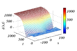
(a) $p=1/R$		(b) $p=R$
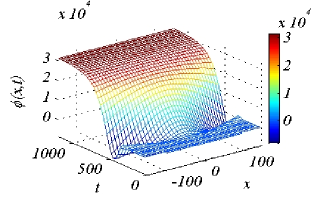
(c) $p=0.0765$		(d) $\phi(x,0)=\delta(x)$

Figure 6: Examples of solutions (15), (16) for $R=146.7126$, which corresponds to $L=40\pi$.

The steady coalescent pole solutions to the Sivashinsky equation correspond to the flame fronts propagating steadily with the velocity exceeding $u_{b}=1$ by $V_{L}$, see e.g. [13]. Addition of the perturbation $\phi(x,t)$ results in a change in the velocity of propagation by the value of the space average of $\partial_{t}\phi$, which we denote $<\!\!\phi_{t}\!\!>$. The correction provided by the $\phi(x,t)$ is only valid in a small vicinity of the crest of $\Phi_{L}(x,t)$ . In sequel, the correction of the speed $<\!\!\phi_{t}\!\!>$ is only valid for a small region $-\varepsilon\leq x\leq\varepsilon$ of the flame front in a vicinity of the crest of $\Phi_{L}(x,t)$. Hence, for our simplified linear model we define the increase of the flame propagation speed as follows:

$$<\!\!\phi_{t}\!\!>=\frac{1}{2\varepsilon}\int\limits_{-\varepsilon}^{\varepsilon}\partial_{t}\phi dx\approx\left.\partial_{t}\phi\right|_{x=0}.$$ (17)

For the single harmonics solution (13) the expression for $<\!\!\phi_{t}\!\!>$ is obvious and is illustrated in Fig. 7. These graphs demonstrate high sensitivity of $<\!\!\phi_{t}\!\!>$ to the wavelength of the perturbation. The phase, or location of the perturbation, is important as well.

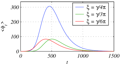
Figure 7: Averaged increase of the local flame propagation speed $<\!\!\phi_{t}\!\!>$ for solutions (13), $\varphi=0$.

4 The effect of noise

According to the results of Section 2, the forcing in the Sivashinsky equation can be decomposed into the most amplifiable nonmodal component and the orthogonal complement. The latter can be neglected reducing spatio-temporal stochastic noise to the appearance of a sequence of the most growing perturbations $\psi_{\alpha_{m}}(x,t^{*})$, $1\leq\alpha_{m}\leq\alpha^{*}=\alpha^{*}(f_{0})$ at a set of time instances $t_{m}$, $m=0,1,2,\ldots$:

$$f(x,t)\approx f_{0}\sum\limits_{m=0}^{\infty}\psi_{\alpha_{m}}(x,t^{*})\delta(t-t_{m}),\qquad 1\leq\alpha_{m}\leq\alpha^{*}=\alpha^{*}(f_{0}).$$ (18)

Thus, the amplitude of noise $f_{0}$, alongside with the averages and the standard deviations of $t_{m+1}-t_{m}$ and $\alpha_{m}$, $m=0,1,2,\ldots$ are the only essential parameters of such a representation of noise.

The impulse-like noise (18) is used here for the sake of simplicity. Some arguments towards its validity were suggested in [2]. More sophisticated and physically realistic models of temporal noise characteristics can be used with (1) as well.

If $f_{0}\ll\sigma_{1}^{-1}(t^{*})$ then noise is not able to affect the flame at all and can be completely neglected. This case can be referred to as the noiseless regime. On the other hand, if $f_{0}$ is comparable with the amplitude $a$ of the background solution $\Phi_{L}(x,t)$, then almost all components of noise will be able to disturb the flame and the $f(x,t)$ in (1) should be treated as a genuine spatio-temporal stochastic function. This is the regime of the saturated noise.

Eventually, there is an important transitional regime when the noise amplitude $f_{0}$ is at least of order of $\sigma_{1}^{-1}(t^{*})$, but still much smaller than $a$. In this case only the disturbances with a significant component in the subspace spanned by the linear combinations of $\psi_{\alpha}(x,t^{*})$, $1\leq\alpha\leq\alpha^{*}$ have a potential to affect the solution. All other disturbances can be neglected and the force $f(x,t)$ in the Sivashinsky equation (1) can be approximated by (18) with a finite value of $\alpha^{*}$. We would like to stress that though such representation of noise is correct for noise of any amplitude, apparently it is only efficient if $f_{0}<\sigma_{\alpha^{*}}^{-1}(t^{*})\ll a$, where $\alpha^{*}$ is small enough.

4.1 Noise in the linear model

A random point-wise set of perturbations uniformly distributed in time and in the Fourier space is a suitable model for both the computational round-off errors and a variety of perturbations of physical origins. We are adopting such a model in our analysis in the following form

$$f(x,t)=\sum\limits_{m=1}^{M(t)}a_{m}\cos(2\pi\xi_{m}x+\varphi_{m})\delta(t-t_{m}),$$ (19)

where $a_{m}$, $t_{m}$, $\xi_{m}$, and $\varphi_{m}$ are non-correlated random sequences. It is assumed that $t_{1}\leq t_{2}\leq\cdots\leq t_{m}\leq\cdots\leq t_{M(t)}\leq t$, $0\leq\varphi_{m}\leq 2\pi$, and $\xi_{m}\geq 0$, $m=1,2,\ldots,M(t)$. Availability of the exact solution (15) makes it also possible to study an alternative noise model based on elementary perturbations $a_{m}e^{-p_{m}(x-x_{m})^{2}}$, which are local in physical space.

Using (11), (12) for the zero initial condition, the exact solution to (9), (19) can be written as

$$\phi(x,t)=\sum\limits_{m=1}^{M(t)}a_{m}e^{-2\pi^{2}R\left[1-e^{-2(t-t_{m})/R}\right]\xi_{m}^{2}+\pi\gamma R\left[1-e^{-(t-t_{m})/R}\right]\xi_{m}}$$

$$\times\cos\left[2\pi\xi_{m}e^{-(t-t_{m})/R}x+\varphi_{m}\right].$$ (20)

The expression for $<\!\!\phi_{t}\!\!>$ is obvious, see (17), and is illustrated in Fig. 8. Here we generated random sequences of the time instances $t_{m}$ with a given frequency $F=M(T)/T$ on a time interval $t\in[0,T]$. Values of the wave number $\xi_{m}$ and of the amplitude $a_{m}$ were also randomly generated and uniformly distributed within certain ranges. According to the formula for $<\!\!\phi_{t}\!\!>$, the effect of the phase shift $\varphi_{m}$ just duplicates the $a_{m}$. Therefore, its value was fixed as $\varphi_{m}\equiv 0$.

If values of $a_{m}$ are uniformly distributed in $[-1,1]$, then the time average of $<\!\!\phi_{t}\!\!>$ is obviously zero, because of the linearity of the problem. In the Sivashinsky equation this effect is compensated by the nonlinearity. The cusps generated by the perturbations of opposite signs move into opposite directions along the flame surface, see Section 2, though they both contribute into the speed positively. This effect of the nonlinearity can be mimicked by restricting the range of possible values of the amplitudes, e.g. $a_{m}\in[0,1]$, as this can be seen in Fig. 8.

(a) $F=1$,  $a_{m},\xi_{m}\in[0,1]$	(b) $F=1/33$, $a_{m}\in[0,1]$,
	$\xi_{m}\equiv\gamma/(4\pi)$

Figure 8: The effect of noise (19) on $<\!\!\phi_{t}\!\!>$ for $L=40\pi$.

Figure 8(b) shows that the increase of $<\!\!\phi_{t}\!\!>$ seen in Fig. 8(a) can be matched by using only the largest growing perturbations with much smaller frequency, which is quite expected in virtue of the linearity of the problem. The amplitude of fluctuations in Fig. 8(a) is noticeably less than in Fig. 8(b). This is attributed to the smoothing effect of the less growing perturbations.

Because of the linearity of the problem in question, the effect of $F=M(T)/T$ and $L$ on $<\!\!\phi_{t}\!\!>$ is straightforward. In particular, the value of $<\!\!\phi_{t}\!\!>$ raises up to about $4\times 10^{8}$ for $L=80\pi$ and other parameters the same as in Fig. 8(a). It should be noticed however that because of the limitation $a_{m}\geq 0$ the quantity $<\!\!\phi_{t}\!\!>$ does no longer represent the increase of propagation speed of the flame, but is just a measure of the rate of transient amplification of perturbations. Figure 9 illustrates the point, see also [7] and [12].

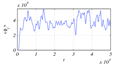
Figure 9: The effect of noise (19) on $<\!\!\phi_{t}\!\!>$ for $L=80\pi$, $F=1$, $a_{m}\in[0,1]$, and $\xi_{m}\in[0,1]$.

Direct studies of the effect of noise in the Sivashinsky equation necessitate use of numerical simulations. However, because of the intrinsic discontinuity of noise, such DNS are hampered with very low accuracy of approximations questioning the validity of numerical solutions. In this work we used explicit solutions (20) in order to validate DNS of (9) and, in sequel, of (1). The DNS of (9), (19) was carried out using a spectral method. The delta function $\delta(t-t_{m})$ was approximated by $(\pi\Delta t)^{-1/2}e^{-(t-t_{m})^{2}/\Delta t}$ with a small enough $\Delta t\ll 1/F$. The calculations have shown that discrepancies between (20) and its numerical counterparts obtained with the same sets of $t_{m}$, $a_{m}$, and $\xi_{m}$ might be noticeable in a neighbourhood of the time instances $t\approx t_{m}$. Although, the averaged characteristics like $<\!\!\phi_{t}\!\!>$ were quite accurate. So, this linear model validates the DNS of the forced Sivashinsky equation at least in relation to the averaged flame propagation speed.

4.2 The Sivashinsky equation

We carried out a series of computations of (1), (18) with $\Phi_{L}(x,t)$ as initial condition and with a variety of parameters of the noise term. Up to twelve basis functions $\psi_{\alpha}(x,10^{3})$, where $\alpha$ was uniformly distributed in the interval $1\leq\alpha\leq\alpha^{*}\leq 12$, were used. The sign of $f_{0}$ in (18) was either plus or minus for every $m$ with the equal probability $1/2$. The delta function $\delta(t-t_{m})$ was approximated by $(\pi\Delta t)^{-1/2}e^{-(t-t_{m})^{2}/\Delta t}$ with a small enough value of $\Delta t$.

The effect of the amplitude of noise on the flame speed is illustrated in Fig. 10. Use of only two basis functions $\psi_{1,2}(x,10^{3})$ gives almost the same result. Similar to the linear model (9) the only noticeable difference was in slightly larger fluctuations of $<\!\!\Phi_{t}\!\!>$. Examples of the effect of composition of noise on $<\!\!\Phi_{t}\!\!>$ are given in Fig. 11 too.

Figure 10: The effect of the amplitude of noise (18) on $<\!\!\Phi_{t}\!\!>$ for $L=40\pi$. Here $F=1/15$ and $\alpha^{*}=12$.

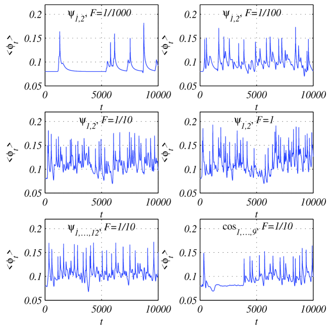
Figure 11: Examples of the effect of the composition of noise on $<\!\!\Phi_{t}\!\!>$ for $f_{0}=10^{-3}$ and $L=40\pi$.

It was mentioned in the previous section that the wave number of the largest Fourier component of $\psi_{1,2}(x,10^{3})$ is exactly the same as the wave number $\xi_{0}=\gamma/(4\pi)$ of the largest growing single harmonics solution to (9). We tried to exploit this observation and simplified (18) even further, replacing $\psi_{\alpha(m)}(x,t^{*})$ by $\cos(\gamma x/4)$, which corresponds to $\xi_{0}$, i.e.

$$f(x,t)\approx f_{0}\cos\frac{\gamma x}{4}\sum\limits_{m=0}^{\infty}\delta(t-t_{m}).$$ (21)

This kind of forcing is able to speed up the flame, but the difference between the computational results obtained with (18) and (21) is noticeable. It does not disappear even if eight nearest sidebands are added to (21), see Fig. 11.

The time averages of $<\!\!\Phi_{t}\!\!>$, denoted here as

$$<\!\!<\!\!\Phi_{t}\!\!>\!\!>=\frac{1}{t_{end}-t_{0}}\int\limits_{t_{0}}^{t_{end}}<\!\!\Phi_{t}\!\!>dt,$$ (22)

are depicted in Fig. 12 versus $F$ (left) and $f_{0}$ (right). Discrepancies in $<\!\!<\!\!\Phi_{t}\!\!>\!\!>$ for different $\alpha^{*}$ did not exceed the variations caused by the different randomly chosen sequences of $t_{m}$. Although, effect of using (21) instead of (18) is appreciable.

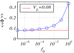
(a) $f_{0}=10^{-3}$	(b) $F=1/15$, $\alpha^{*}=12$,

Figure 12: The effect of the composition (a) and amplitude (b) of noise on the spatio-temporally averaged flame propagation speed $<\!\!<\!\!\Phi_{t}\!\!>\!\!>$. Here $L=40\pi$ and the temporal averaging was over the interval $t\in[200,10^{4}]$.

The correlation between the flame propagation speed and the noise amplitude is obvious. Note that the $f_{0}$ in the right most point in the graph is still about $20$ times less than the amplitude of the variation of the background solution $\Phi_{L}(x,t)$.

In accordance with the idea developed in this paper, the value of $<\!\!<\!\!\Phi_{t}\!\!>\!\!>$ is determined by the product $\sigma_{1}f_{0}$. It was shown in [7] that $\sigma_{1}\propto e^{O(L)}$, resulting in $<\!\!<\!\!\Phi_{t}\!\!>\!\!>=<\!\!<\!\!\Phi_{t}\!\!>\!\!>(e^{O(L)}f_{0})$. Thus, the data shown in Fig. 12 are at least in a qualitative agreement with the dependence of $<\!\!<\!\!\Phi_{t}\!\!>\!\!>$ on $L$, which was obtained in [7] for a fixed noise amplitude $f_{0}\approx 10^{-16}$ associated with the computational round-off errors.

Eventually, in Fig. 13 we presented the results of an attempt to control the flame propagation speed using our special perturbations $\psi_{\alpha}(x,t^{*})$ of properly selected amplitudes. Graphs of $<\!\!\Phi_{t}\!\!>$ and $<\!\!<\!\!\Phi_{t}\!\!>\!\!>$ are shown in the left and numerical solution $\Phi(x,t)$ corresponding to this controlling experiment is illustrated in the right. The fluctuations of the obtained flame propagation speed are large indeed, but at least, they appear in quite a regular pattern.

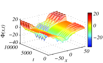
Figure 13: An example of controlling the flame speed with the amplitude of the perturbations $f_{0}$. Here $F=1/15$, $\alpha^{*}=12$, and $L=40\pi$.

In this paper noise or forcing in (1) represents the turbulence of the upstream velocity field, which is difficult to manage in practice. The controlling function is more effectively achieved by acoustic signals, see e.g. [14]. Acoustics was neglected in the evaluation of the Sivashinsky equation and there is no easy and straightforward way to incorporate it back into the model. However, because of a strong coupling between the velocity and pressure fields, effects of acoustic signals similar to those presented here can be expected as well.

5 Conclusions

Based on our analysis of the steadily propagating cellular flames governed by the Sivashinsky equation we may conclude that there are perturbations of very small amplitude, which can essentially affect the flame front dynamics. The subspace formed by these special perturbations is of a very small dimension and its basis can be used for an efficient representation of the upstream velocity turbulence. These are the very perturbations which cause the increase of the flame propagation speed in numerical experiments. Hence, theoretically, they can be used to model certain regimes of flame-turbulence interaction and to control the flame propagation speed on purpose.

References

- [1] G.I. Sivashinsky. Acta Astronautica, 4:1177–1206, 1977.
- [2] G. Joulin. Combust. Sci. Tech., 60:1–5, 1988.
- [3] G. Joulin and P. Cambray. Combust. Sci. Tech., 81:243–256, 1992.
- [4] P. Cambray and G. Joulin. 24th Symp (Int) Combust, 61–67, Combust Inst, 1992.
- [5] O. Thual, U. Frisch, and M. Hénon. Le J. de Phys., 46(9):1485–1494, 1985.
- [6] D. Vaynblat and M. Matalon. SIAM J. Appl. Math., 60(2):679–702, 2000.
- [7] V. Karlin. Proc. Combust. Inst., 29(2):1537–1542, 2002.
- [8] G. Joulin. J. Phys. France, 50:1069–1082, 1989.
- [9] I.C. Gohberg and M.G. Krein. Introduction to the Theory of Linear Nonselfadjoint Operators. AMS, Providence, Rhode Island, 1969.
- [10] V. Karlin. Math. Meth. Model. Appl. Sci., 14(8):1191–1210, 2004. (Preprint arXiv: physics/0312095, December, 2003 at http://arxiv.org).
- [11] G.H. Golub and C.F. van Loan. Matrix Computations. The Johns Hopkins University Press, 1989.
- [12] V. Karlin, V. Maz’ya, and G. Schmidt. J. Comput. Phys., 188(1):209–231, 2003.
- [13] M. Rahibe, N. Aubry, and G.I. Sivashinsky. Combust. Theory Modelling, 2(1):19–41, 1998.
- [14] C. Clanet and G. Searby. Physical Review Letters, 80(17):3867–3870, 1998.