First-Principles Method for Open Electronic Systems

Abstract

We prove the existence of the exact density-functional theory formalism for open electronic systems, and develop subsequently an exact time-dependent density-functional theory (TDDFT) formulation for the dynamic response. The TDDFT formulation depends in principle only on the electron density of the reduced system. Based on the nonequilibrium Green’s function technique, it is expressed in the form of the equation of motion for the reduced single-electron density matrix, and this provides thus an efficient numerical approach to calculate the dynamic properties of open electronic systems. In the steady-state limit, the conventional first-principles nonequilibrium Green’s function formulation for the current is recovered.

Density-functional theory (DFT) has been widely used as a research tool in condensed matter physics, chemistry, materials science, and nanoscience. The Hohenberg-Kohn theorem hk lays the foundation of DFT. The Kohn-Sham formalism ks provides the practical solution to calculate the ground state properties of electronic systems. Runge and Gross extended further DFT to calculate the time-dependent properties and hence the excited state properties of any electronic systems tddft . The accuracy of DFT or TDDFT is determined by the exchange-correlation functional. If the exact exchange-correlation functional were known, the Kohn-Sham formalism would have provided the exact ground state properties, and the Runge-Gross extension, TDDFT, would have yielded the exact properties of excited states. Despite of their wide range of applications, DFT and TDDFT have been mostly limited to closed systems.

Fundamental progress has been made in the field of molecular electronics recently. DFT-based simulations on quantum transport through individual molecules attached to electrodes offer guidance for the design of practical devices prllang ; prlheurich ; jcpluo . These simulations focus on the steady-state currents under the bias voltages. Two types of approaches have been adopted. One is the Lippmann-Schwinger formalism by Lang and coworkers langprb . The other is the first-principles nonequilibrium Green’s function technique prbguo ; jacsywt ; jacsgoddard ; transiesta ; jcpratner . In both approaches the Kohn-Sham Fock operator is taken as the effective single-electron model Hamiltonian, and the transmission coefficients are calculated within the noninteracting electron model. It is thus not clear whether the two approaches are rigorous. Recently Stefanucci and Almbladh derived an exact expression for time-dependent current in the framework of TDDFT qttddft . In the steady-current limit, their expression leads to the conventional first-principles nonequilibrium Green’s function formalism if the TDDFT exchange-correlation functional is adopted. However, they did not provide a feasible numerical formulation for simulating the transient response of molecular electronic devices. In this communication, we present a rigorous first-principles formulation to calculate the dynamic properties of open electronic systems. We prove first a theorem that the electron density distribution of the reduced system determines all physical properties or processes of the entire system. The theorem lays down the foundation of the first-principles method for open systems. We present then the equation of motion (EOM) for nonequilibrium Green’s functions (NEGF) in the framework of TDDFT. By introducing a new functional for the interaction between the reduced system and the environment, we develop further a reduced-single-electron-density-matrix-based TDDFT formulation. Finally, we derive an exact expression for the current which leads to the existing DFT-NEGF formula in the steady-state limit. This shows that the conventional DFT-NEGF formalism can be exact so long as the correct exchange-correlation functional is adopted.

Both Hohenberg-Kohn theorem and Runge-Gross extension apply to isolated systems. Applying Hohenberg-Kohn-Sham’s DFT and Runge-Gross’s TDDFT to open systems requires in principle the knowledge of the electron density distribution of the total system which consists of the reduced system and the environment. This presents a major obstacle in simulating the dynamic processes of open systems. Our objective is to develop an exact DFT formulation for open systems. In fact, we are interested only in the physical properties and processes of the reduced system. The environment provides the boundary conditions and serves as the current source and energy sink. We thus concentrate on the reduced system.

Any electron density distribution function $\rho(\mathbf{r})$ of a real physical system is a real analytic function. We may treat nuclei as point charges, and this would only lead to non-analytic electron density at isolated points. In practical quantum mechanical simulations, analytic functions such as Gaussian functions and plane wave functions are adopted as basis sets, which results in analytic electron density distribution. Therefore, we conclude that any electron density functions of real systems are real analytic on connected physical space. Based on this, we show below that for a real physical system the electron density distribution function on a sub-space determines uniquely its values on the entire physical space. This is nothing but the analytic continuation of a real analytic function. The proof for the univariable real analytical functions can be found in textbooks, for instance, reference proof1 . The extension to the multivariable real analytical functions is straightforward.

Lemma: The electron density distribution function $\rho(\mathbf{r})$ is real analytic on a connected physical space $U$. $W\subseteq U$ is a sub-space. If $\rho(\mathbf{r})$ is known for all $\mathbf{r}\in W$, $\rho(\mathbf{r})$ can be uniquely determined on entire $U$.

Proof: To facilitate our discussion, the following notations are introduced. Set $\mathbb{Z}^{+}=\{0,1,2,\ldots\}$, and $\gamma$ is an element of $(\mathbb{Z}^{+})^{3}$, i.e., $\gamma=(\gamma_{1},\gamma_{2},\gamma_{3})\in(\mathbb{Z}^{+})^{3}$. The displacement vector $\mathbf{r}$ is denoted by the three-dimensional variable $x=(x_{1},x_{2},x_{3})\in U$. Denote that $\gamma\,\mbox{!}=\gamma_{1}\,\mbox{!}\>\gamma_{2}\,\mbox{!}\>\gamma_{3}\,\mbox{!}\,$, $x^{\gamma}=x_{1}^{\gamma_{1}}\>x_{2}^{\gamma_{2}}\>x_{3}^{\gamma_{3}}$, and $\frac{\partial^{\gamma}}{\partial x^{\gamma}}=\frac{{\partial}^{\gamma_{1}}}{\partial x_{1}^{\gamma_{1}}}\frac{\partial^{\gamma_{2}}}{\partial x_{2}^{\gamma_{2}}}\frac{\partial^{\gamma_{3}}}{\partial x_{3}^{\gamma_{3}}}$.

Suppose that another density distribution function $\rho^{\prime}(x)$ is real analytic on $U$ and equal to $\rho(x)$ for all $x\in W$. We have $\frac{\partial^{\gamma}\rho(x)}{\partial x^{\gamma}}=\frac{\partial^{\gamma}\rho^{\prime}(x)}{\partial x^{\gamma}}$ for all $x\in W$ and $\gamma\in(\mathbb{Z}^{+})^{3}$. Taking a point $x_{0}$ at or infinitely close to the boundary of $W$, we may expand $\rho(x)$ and $\rho(x^{\prime})$ around $x_{0}$, i.e., $\rho(x)=\sum_{\gamma\in(\mathbb{Z}^{+})^{3}}\frac{1}{\gamma!}\left.\frac{\partial^{\gamma}\rho(x)}{\partial x^{\gamma}}\right|_{x_{0}}(x-x_{0})^{\gamma}$ and $\rho^{\prime}(x)=\sum_{\gamma\in(\mathbb{Z}^{+})^{3}}\frac{1}{\gamma!}\left.\frac{\partial^{\gamma}\rho^{\prime}(x)}{\partial x^{\gamma}}\right|_{x_{0}}(x-x_{0})^{\gamma}$. Assuming that the convergence radii for the Taylor expansions of $\rho(x)$ and $\rho^{\prime}(x)$ at $x_{0}$ are both larger than a positive finite real number $b$, we have thus $\rho(x)=\rho^{\prime}(x)$ for all $x\in D_{b}(x_{0})=\left\{x:\left|x-x_{0}\right|<b\right\}$ since $\left.\frac{\partial^{\gamma}\rho(x)}{\partial x^{\gamma}}\right|_{x_{0}}=\left.\frac{\partial^{\gamma}\rho^{\prime}(x)}{\partial x^{\gamma}}\right|_{x_{0}}$. Therefore, the equality $\rho^{\prime}(x)=\rho(x)$ has been expanded beyond $W$ to include $D_{b}(x_{0})$. Since $U$ is connected the above procedure can be repeated until $\rho^{\prime}(x)=\rho(x)$ for all $x\in U$.

We have thus proven that $\rho$ can be uniquely determined on $U$ once it is known on $W$, and are ready to prove the following theorem.

Theorem: Electron density function $\rho(\mathbf{r})$ for a subsystem of a connected real physical system determines uniquely all electronic properties of the entire system.

Proof: Assuming the physical space spanned by the subsystem and the real physical system are $W$ and $U$, respectively. $W$ is thus a sub-space of $U$, i.e., $W\subseteq U$. According to the above lemma, $\rho(\mathbf{r})$ on $W$ determines uniquely its values on $U$, i.e., $\rho(\mathbf{r})$ of the subsystem determines $\rho(\mathbf{r})$ of the entire system.

Hohenberg-Kohn theorem and Runge-Gross extension state that the electron density distribution of a system determines uniquely all its electronic properties. Therefore, we conclude that $\rho(\mathbf{r})$ for a subsystem determines all the electronic properties of the real physical system.

The above theorem guarantees the existence of an exact DFT-type method for open systems. In principle, all we need to know is the electron density of the reduced system. The electron density distribution in the environment can be obtained by the analytic continuation of the electron density function at or near the boundary. The challenge is to develop a practical first-principles method.

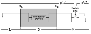
Figure 1: Schematic representation of the experimental setup for quantum transport through a molecular device.

Fig. 1 depicts one type of open systems, a molecular device. It consists of the reduced system or device region $D$ and the environment, the left and right electrodes $L$ and $R$. Taking this as an example, we develop an exact DFT formalism for the open systems. To calculate the properties of a molecular device, we need only the electron density distribution in the device region. The influence of the electrodes can be determined by the electron density distribution in the device region. Within the TDDFT formulation, we proceed to derive the EOM for the lesser Green’s function:

$$G^{<}_{nm}(t,t^{\prime})=i\left\langle a^{\dagger}_{m}(t^{\prime})\,a_{n}(t)\right\rangle,$$ (1)

where $a_{n}(t)$ and $a^{\dagger}_{m}(t^{\prime})$ are the Heisenberg annihilation and creation operators for atomic orbitals $n$ and $m$ in the reduced system $D$ at time $t$ and $t^{\prime}$, respectively. Based on the Keldysh formalism keldysh and the analytic continuation rules of Langreth langreth , Jauho et al. developed a NEGF formulation for current evaluation prb94win . Based on the same procedure adopted in reference prb94win , we obtain

$$i\frac{\partial G^{<}_{nm}(t,t^{\prime})}{\partial t} = \sum_{l\in D}h_{nl}(t)G^{<}_{lm}(t,t^{\prime})$$ (2)

$$+\sum_{l\in D}\int_{-\infty}^{\infty}d\tau\Big{[}\Sigma^{<}_{nl}(t,\tau)G^{a}_{lm}(\tau,t^{\prime})$$

$$+\Sigma^{r}_{nl}(t,\tau)G^{<}_{lm}(\tau,t^{\prime})\Big{]},$$

where $G^{a}_{lm}(\tau,t^{\prime})$ is the advanced Green’s function prbguo , $\Sigma^{<}_{nl}(t,\tau)$ and $\Sigma^{r}_{nl}(t,\tau)$ are the self-energies on $D$ induced by $L$ and $R$ whose expressions can be found in references such as prbguo or prb94win , and $h_{nl}(t)$ is the Kohn-Sham Fock matrix element. Eq. (2) is the exact TDDFT formulation for the open electronic systems. However, $G^{<}_{nm}(t,t^{\prime})$ and $G^{a}_{lm}(\tau,t^{\prime})$ are the two-time Green’s functions. It is thus extremely time-consuming to solve Eq. (2) numerically. Alternative must be sought.

Yokojima et al. developed a dynamic mean-field theory for dissipative interacting many-electron systems yokojima . An EOM for the reduced single-electron density matrix was derived to simulate the excitation and nonradiative relaxation of a molecule embedded in a thermal bath. This is in analogy to our case although our environment is actually a fermion bath instead of a boson bath. The major difference is that the number of electrons in the reduced system is conserved in reference yokojima while in our case it is not. Note that the reduced single-electron density matrix $\sigma$ is actually the lesser Green’s function of identical time variables,

$$\sigma_{nm}(t)=\left.-iG^{<}_{nm}(t,t^{\prime})\right|_{t^{\prime}=t}.$$ (3)

Thus, the EOM for $\sigma$ can be written down readily with the aid of Eq. (2),

$$i\dot{\sigma_{nm}} = \left.\frac{\partial}{\partial t}G^{<}_{nm}(t,t^{\prime})\right|_{t^{\prime}=t}+\left.\frac{\partial}{\partial t^{\prime}}G^{<}_{nm}(t,t^{\prime})\right|_{t^{\prime}=t}$$ (4)

$$= \sum_{l\in D}\left(h_{nl}\sigma_{lm}-\sigma_{nl}h_{lm}\right)+\!\!\!\sum_{\alpha=L,R}\!\!Q_{\alpha,nm}(t),$$

where $Q_{\alpha,nm}(t)$ on the right-hand side (RHS) is the dissipative term due to the lead $\alpha$ ($L$ or $R$) whose expanded form is

$$Q_{\alpha,nm}(t) = i\sum_{l\in D}\int_{-\infty}^{\infty}d\tau\bigg{[}G^{<}_{nl}(t,\tau)\Sigma^{a}_{\alpha,lm}(\tau,t)$$ (5)

$$+\,G^{r}_{nl}(t,\tau)\Sigma^{<}_{\alpha,lm}(\tau,t)-\Sigma^{<}_{\alpha,nl}(t,\tau)G^{a}_{lm}(\tau,t)$$

$$-\,\Sigma^{r}_{\alpha,nl}(t,\tau)G^{<}_{lm}(\tau,t)\bigg{]}.$$

And the current through the interfaces $S_{L}$ or $S_{R}$ (see Fig. 1) can be expressed as

$$J_{\alpha}(t) = -\frac{d}{dt}\left\langle\sum_{k\in\alpha}c^{\dagger}_{k_{\alpha}}\!(t)\,c_{k_{\alpha}}\!(t)\right\rangle$$ (6)

$$= \sum_{k\in\alpha}\sum_{l\in D}\left[V_{l,k_{\alpha}}^{\ast}(t)G^{<}_{l,k_{\alpha}}(t,t)-G^{<}_{k_{\alpha},l}(t,t)V_{l,k_{\alpha}}(t)\right]$$

$$= 2\Re\bigg{\{}\int_{-\infty}^{\infty}d\tau\,\textnormal{tr}\Big{[}G^{<}_{D}(t,\tau)\Sigma^{a}_{\alpha}(\tau,t)$$

$$+\,G^{r}_{D}(t,\tau)\Sigma^{<}_{\alpha}(\tau,t)\Big{]}\bigg{\}}$$

$$= -i\,\mbox{tr}\bigg{[}Q_{\alpha}(t)\bigg{]}=-i\sum_{n\in D}Q_{\alpha,nn}(t),$$

where $V_{l,k_{\alpha}}(t)$ is the coupling matrix element between the atomic orbital $l$ and the single-electron state $k_{\alpha}$ in $L$ or $R$, $G^{<}_{k_{\alpha},l}(t,t^{\prime})\equiv i\langle a^{\dagger}_{l}(t^{\prime})\,c_{k_{\alpha}}\!(t)\rangle$ and $G^{<}_{l,k_{\alpha}}(t,t^{\prime})\equiv i\langle c^{\dagger}_{k_{\alpha}}\!(t^{\prime})\,a_{l}(t)\rangle$, $c_{k_{\alpha}}\!(t)$ and $c^{\dagger}_{k_{\alpha}}\!(t^{\prime})$ are the annihilation and creation operators for $k_{\alpha}$, respectively. At first glance Eq. (4) is not self-closed since the $G$s are to be solved. According to the theorem we proved earlier, all physical quantities are explicit or implicit functionals of the electron density in $D$, $\rho_{D}(t)$. $G$s and $\Sigma$s are thus also universal functionals of $\rho_{D}(t)$. Therefore, we can recast Eq. (4) into a formally closed form,

$$i\dot{\sigma}=\Big{[}h[\rho_{D}(t)],\sigma\Big{]}+\sum_{\alpha=L,R}Q_{\alpha}[\rho_{D}(t)].$$ (7)

Neglecting the second term on the RHS of Eq. (7) leads to the conventional TDDFT formulation in terms of reduced single-electron density matrix ldmtddft . The second term describes the dissipative processes where electrons enter and leave the region $D$. Besides the exchange-correlation functional, the additional universal density functional $Q_{\alpha}[\rho_{D}(t)]$ is introduced to account for the dissipative interaction between the reduced system and its environment. Eq. (7) is thus the TDDFT formulation in terms of the reduced single-electron matrix for the open system. In the frozen DFT approach warshel an additional exchange-correlation functional term was introduced to account for the exchange-correlation interaction between the system and the environment. This additional term is included in $h[\rho_{D}(t)]$ of Eq. (7). Admittedly, $Q_{\alpha}[\rho_{D}(t)]$ can be an extremely complex functional. Progressive approximations are needed for the practical solution of Eq. (7). Compared to Eq. (2), Eq. (7) may be much more convenient to be solved numerically.

To obtain the steady-state solution of Eqs. (4) or (7), we adopt a similar strategy as that of reference qttddft . As $t,\tau\rightarrow+\infty$, $\Gamma^{k_{\alpha}}_{nm}(t,\tau)=V_{n,k_{\alpha}}\!(t)V_{m,k_{\alpha}}^{\ast}\!(\tau)$ becomes asymptotically time-independent, and $G$s and $\Sigma$s rely simply on the difference of the two time-variables qttddft . The expression for the steady-state current is thus as follows,

$$J_{L}(\infty) = -J_{R}(\infty)=-i\sum_{n\in D}Q_{L,nn}(\infty)$$ (8)

$$= \int\left[f^{L}(\epsilon)-f^{R}(\epsilon)\right]T(\epsilon)\,d\epsilon,$$

$$T(\epsilon) = 2\pi\eta_{L}(\epsilon)\eta_{R}(\epsilon)$$ (9)

$$\times\,\mbox{tr}\Big{[}G^{r}_{D}(\epsilon)\Gamma^{R}(\epsilon)G^{a}_{D}(\epsilon)\Gamma^{L}(\epsilon)\Big{]}.$$

Here $T(\epsilon)$ is the transmission coefficient, $f^{\alpha}(\epsilon)$ is the Fermi distribution function, and $\eta_{\alpha}(\epsilon)=\sum_{k\in\alpha}\delta(\epsilon-\varepsilon^{\alpha}_{k})$ is the density of states for the lead $\alpha$ ($L$ or $R$). Eq. (8) is exactly the Landauer formula bookdatta ; landauer in the DFT-NEGF formalism prbguo ; jacsywt . The only difference is that Eq. (8) is derived within the TDDFT formalism in our case while it is evaluated within the DFT framework in the case of the DFT-NEGF formulation prbguo ; jacsywt . In other words, the DFT-NEGF formalism can be exact so long as the correct exchange-correlation functional is used! This is not surprising, and is simply a consequence of that (i) DFT and TDDFT can yield the exact electron density and (ii) the current is the time derivative of the total charge.

Just as the exchange-correlation functional, the exact functional form of $Q_{\alpha}$ on density is rather difficult to derive. Various approximated expressions have been adopted for the DFT exchange-correlation functional in the practical implementation. Similar strategy can be employed for $Q_{\alpha}$. One such scheme is the wide-band limit (WBL) approximation prb94win , which consists of a series of approximations imposed on the leads: (i) their band-widths are assumed to be infinitely large, (ii) their linewidths $\Lambda^{\alpha}_{k}(t,\tau)$ defined by $\pi\eta_{\alpha}(\varepsilon^{\alpha}_{k})\Gamma^{k_{\alpha}}(t,\tau)$ are regarded as energy independent, i.e., $\Lambda^{\alpha}_{k}(t,\tau)\approx\Lambda^{\alpha}(t,\tau)\approx\Lambda^{\alpha}$, and (iii) the energy shifts are taken as level independent, i.e., $\delta\varepsilon^{\alpha}_{k}(t)\approx\delta\varepsilon^{\alpha}(t)\approx\delta\varepsilon^{\alpha}$ for $L$ or $R$. The physical essence of the transport problem is captured under these reasonable hypotheses prb94win . In the practical implementation, the effects of the specific electronic structures of the leads can be captured by enlarging the device region to include enough portions of the electrodes.

Following the WBL approximation in reference prb94win , we obtain that

$$Q_{\alpha}=\left[P^{\alpha}(t)-\left[P^{\alpha}(t)\right]^{\dagger}\right]-i\left\{\Lambda^{\alpha},\sigma\right\},$$ (10)

where the curly bracket on the RHS denotes the anticommutator, and by taking $t=0$ as the switch-on instant $P^{\alpha}(t)$ can be expressed as

$$P^{\alpha}(t) = \frac{2}{\pi}\,U^{(-)}(t)\Bigg{\{}\!\int_{0}^{t}d\tau\,\frac{\mbox{e}^{\,i\left(\mu^{\alpha\!,\,0}+\delta\varepsilon^{\alpha}\right)(t-\tau)}}{t-\tau}\,U^{(+)}(\tau)$$ (11)

$$+\!\int_{-\infty}^{0}\!\!d\tau\,\frac{i\,\mbox{e}^{\,i\left[\delta\varepsilon^{\alpha}t+\mu^{\alpha\!,\,0}(t-\tau)\right]}}{t-\tau}\,G^{r,0}_{D}(-\tau)\!\Bigg{\}}\Lambda^{\alpha}$$

$$+\,2i\,\Lambda^{\alpha},$$

where $\mu^{\alpha\!,\,0}$ is the chemical potential of the lead $\alpha$ ($L$ or $R$) in its initial ground state, $G^{r,\,0}_{D}(-\tau)$ is the retarded Green’s function of $D$ before the switch-on instant, and $U$s are defined as

$$U^{(\pm)}(t) = \exp\bigg{\{}\pm i\int_{0}^{t}\!h(\tau)d\tau\pm\!\!\sum_{\alpha=L,R}\Lambda^{\alpha}t\bigg{\}}.$$ (12)

Eqs. (10)$-$(12) constitute the WBL formulation of the TDDFT-NEGF formalism. Although its explicit functional dependency is not given, $Q_{\alpha}$ depends implicitly on $\rho_{D}$ via Eqs. (10)$-$(12).

To summarize, we have proven the existence of the exact TDDFT formalism for the open electronic systems, and have proposed a TDDFT-NEGF formulation to calculate the quantum transport properties of molecular devices. Since TDDFT results in formally exact density distribution, the TDDFT-NEGF formulation is in principle an exact theory to evaluate the transient and steady-state currents. In particular, the TDDFT-NEGF expression for the steady-state current has the exact same form as that of the conventional DFT-NEGF formalism prbguo ; jacsywt ; jacsgoddard ; transiesta ; jcpratner , and this provides rigorous theoretical foundation for the existing DFT-based methodologies langprb ; prbguo ; jacsywt ; jacsgoddard ; transiesta ; jcpratner calculating the steady currents through molecular devices.

In addition to the conventional exchange-correlation functional, a new density functional is introduced to account for the dissipative interaction between the reduced system and the environment. In the WBL approximation, the new functional can be expressed in a relatively simple form which depends implicitly on the electron density of the reduced system. Since the basic variable in our formulation is the reduce single-electron density matrix, the linear-scaling techniques such as that of reference ldmtddft can be adopted to further speed up the computation.

Authors would thank Hong Guo, Jiang-Hua Lu, Jian Wang, Arieh Warshel and Weitao Yang for stimulating discussions. Support from the Hong Kong Research Grant Council (HKU 7010/03P) and the Committee for Research and Conference Grants (CRCG) of The University of Hong Kong is gratefully acknowledged.

References

- (1)
- (2) P. Hohenberg and W. Kohn, Phys. Rev. 136, B 864, (1964)
- (3) W. Kohn and L. J. Sham, Phys. Rev. 140, A 1133 (1965)
- (4) E. Runge and E. K. U. Gross, Phys. Rev. Lett. 52, 997 (1984)
- (5) N. D. Lang and Ph. Avouris, Phys. Rev. Lett. 84, 358 (2000)
- (6) J. Heurich, J. C. Cuevas, W. Wenzel and G. Schön, Phys. Rev. Lett. 88, 256803 (2002)
- (7) C.-K. Wang and Y. Luo, J. Chem. Phys. 119, 4923 (2003)
- (8) N. D. Lang, Phys. Rev. B 52, 5335 (1995)
- (9) J. Taylor, H. Guo and J. Wang, Phys. Rev. B. 63, 245407 (2001)
- (10) S.-H. Ke, H. U. Baranger and W. Yang, J. Am. Chem. Soc. 126, 15897 (2004)
- (11) W.-Q. Deng, R. P. Muller and W. A. Goddard III, J. Am. Chem. Soc. 126, 13563 (2004)
- (12) M. Brandbyge et al., Phys. Rev. B 65, 165401 (2002)
- (13) Y. Xue, S. Datta and M. A. Ratner, J. Chem. Phys. 115, 4292 (2001)
- (14) G. Stefanucci and C.-O. Almbladh, Europhys. Lett. 67 (1), 14 (2004)
- (15) S. G. Krantz and H. R. Parks, A Primer of Real Analytic Functions, Birkhuser Boston (2002)
- (16) L. V. Keldysh, JETP 20, 1018 (1965)
- (17) D. C. Langreth and P. Nordlander, Phys. Rev. B 43, 2541 (1991)
- (18) A.-P. Jauho, N. S. Wingreen and Y. Meir, Phys. Rev. B 50, 5528 (1994)
- (19) S. Yokojima, G.H. Chen, R. Xu and Y. Yan, Chem. Phys. Lett. 369, 495 (2003); J. Comp. Chem. 24, 2083 (2003)
- (20) C. Y. Yam, S. Yokojima and G.H. Chen, J. Chem. Phys. 119, 8794 (2003); Phys. Rev. B 68, 153105 (2003)
- (21) T. A. Wesolowski and A. Warshel, J. Phys. Chem. 97, 8050 (1993)
- (22) S. Datta, Electronic Transport in Mesoscopic Systems, Cambridge University Press (1995)
- (23) R. Landauer, Philos. Mag. 21, 863 (1970)