New distributed offline processing scheme at Belle
Abstract
The offline processing of the data collected by the Belle detector has been recently upgraded to cope with the excellent performance of the KEKB accelerator. The 127 fb-1 of data (120 TB on tape) collected between autumn 2003 and summer 2004 has been processed in 2 months, thanks to the high speed and stability of the new, distributed processing scheme. We present here this new processing scheme and its performance.
1 INTRODUCTION
The Belle experiment [1], located on the KEKB [2] asymmetric-energy collider, is primarily devoted to the study of CP violation in the meson system. KEKB has shown a very stable operation with increasing luminosity over the years. It has turned to so-called “continuous injection mode” last January, thus allowing a gain in the integrated luminosity of about 30%. In this mode, the beam particle losses are compensated by continuously injecting beam from the linear accelerator, without interruption of data taking.
KEKB has reached a world record peak luminosity of cm-2s-1 and an integrated luminosity of about 1 fb-1 per day. In the meanwhile, Belle has accumulated a total integrated luminosity of 290 fb-1 (about 275 million meson pairs), among which 127 fb-1 was collected between October 2003 and July 2004 (SVD2 run).
| DAQ output rate | 8.9 MB/s | |
|---|---|---|
| Raw event size | 38 kB | |
| DST event size | 60 kB | |
| mdst event size | 12 kB | |
| Total raw data | 247 TB | (120 TB) |
| Total DST data | 390 TB | (186 TB) |
| Total mdst data | 80 TB | (40 TB) |
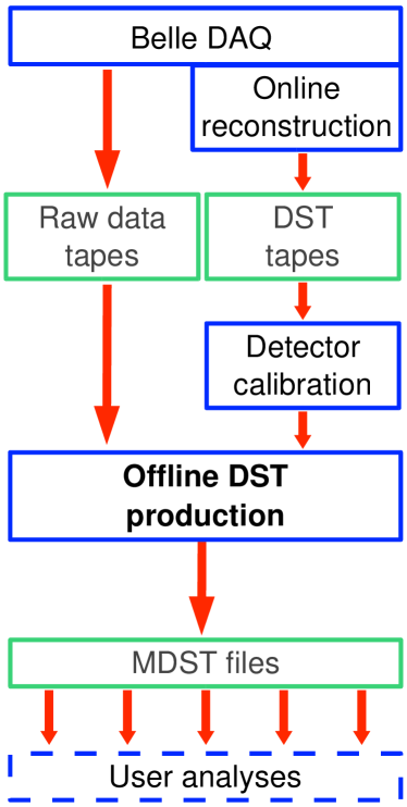
A (simplified) overview of the Belle data flow is shown in Figure 1. The subdetector information is collected by the Belle data acquisition (DAQ) at an average output rate of about 230 events per second. This raw data is stored on tapes and is, at the same time, processed by the online reconstruction farm [3] (RFARM). The data processed by the RFARM is stored to data summary tapes (DST) and is used for detector calibration. The offline DST processing then reads in the raw data tapes and uses the calibration constants to produce mini-DST (mdst) files, which are used for physics analyses. The main figures of the data flow are summarized in Table 1.
In this paper, we present the new offline processing scheme used to process the data collected during SVD2 run. We first introduce the computing hardware and software tools. An overview and the performance of the processing scheme are then given.
2 COMPUTING HARDWARE
The hardware used for DST processing consists of storage systems and computing farms detailed below. The components are connected together by Gigabit ethernet switches.
2.1 Data Storage
Two types of data storage are used.
Raw and DST data is stored on SONY DTF2 tapes (200 GB tapes), providing a total storage space of 500 TB. They are accessed through 20 tape servers (Solaris mainframe servers with 4 CPUs at 0.5 GHz each), each server being connected to two tape drives with a maximum readout rate of 24 MB/s.
Mdst data is stored on a new hierarchical storage management system [4] (HSM) provided by SONY. It consists of a hybrid disk and tape storage system with 500 GB tapes and 1.6 TB RAID disks. The total tape storage space is 450 TB (to be soon expanded to 1.2 PB), while disk space reaches 26 TB in total. The tapes are readout by SONY SAIT tapes with a maximum rate of 30 MB/s. The 16 disks are connected to 8 servers with 4 CPUs at 2.8 GHz each. The data stored on disk is automatically migrated to the tapes by the HSM system. Unused data is deleted from the disks and automatically reloaded when accessed by users.
2.2 Computing Farms
The DST processing was performed on three classes of PC farms: {Itemize}
Class I farm: 60 hosts with 4 Intel Xeon CPUs at 0.766 GHz each (16.4% of total power).
Class II farm: 119 hosts with 2 Intel Pentium III CPUs at 1.26 GHz each (26.7% of total power).
Class III farm: 100 hosts with 2 Intel Xeon CPUs at 3.2 GHz each (56.9% of total power).
The total available CPU power is 1.12 THz, distributed among 279 hosts. These are divided into 8 different clusters of 30 to 40 hosts.
3 SOFTWARE TOOLS
The DST processing scheme makes use of a number of software tools. The core software is based on three “home-grown” tools detailed below. Other tools are also mentioned.
3.1 The Belle Analysis Software Framework
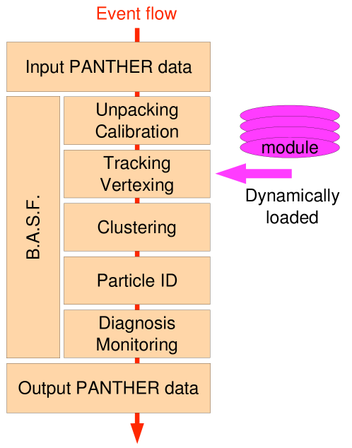
B.A.S.F. is the software framework used for all Belle data analyses, from data acquisition to end-user analysis and DST processing. It provides an interface to external programs (modules), dynamically loaded as shared objects at the start of a processing job. The interface includes begin and end run calls, event calls, histogram definitions, as well as a shared memory utility. External modules actually process the event information. Several modules can be called at will, in the order specified by the user. B.A.S.F. is written in C++ (and so are the modules). Finally, B.A.S.F. supports Symmetrical Multiprocessing (SMP), thus allowing parallel processing of events on a multi-processor machine. Figure 2 shows the event flow for a DST processing job.
3.2 Network Shared Memory
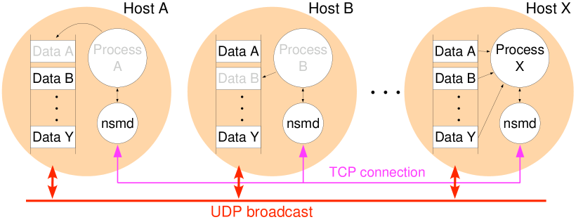
The NSM package provides tools for information exchange over a TCP/IP based LAN. It allows processes running on different machines to share memory across the network, or send requests and messages to each other.
3.3 The PANTHER format
The input and output of Belle data, as well as transfer between modules, is managed by the PANTHER system. It is used consistently from raw data to user analysis. The PANTHER format consists of compressed tables (banks), using the standard zlib libraries. A cross-reference system is implemented in order to allow navigation between the tables. The table formats are defined in B.A.S.F. in ASCII header files, which are loaded before the modules. Users may define their own tables.
3.4 Other tools
In addition to the software described above, DST processing uses various other standard tools:
The postgresql database system [5]. An important part of the information relevant to DST processing is stored in databases: calibration constants; meta-data information about raw data, DST and mdst files; tapes and tape drives information; PC farms description. The DST processing uses a dedicated postgresql server mirrored from the main database server.
LSF batch queues [6]. Tape servers are operated through the LSF queuing system.
4 DST PROCESSING SCHEME
The new DST processing scheme has been implemented between March and May 2004. It is based on a distributed version of B.A.S.F., dbasf, first developed for the online processing (RFARM) and adapted to the configuration of offline processing. The computing facility used for DST processing was divided in a number of dbasf clusters (see sub-section Computing Farms above) that independently process groups of events (runs). The processing is fully managed by a steering Perl script (dcruncher) that allocates jobs and surveys the global DST processing operations.
4.1 Distributed B.A.S.F.
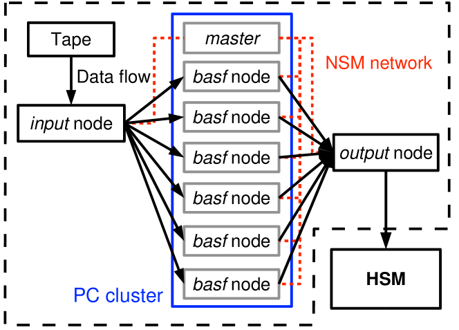
In order to increase its parallel-processing ability, B.A.S.F. was extended to a distributed version that relies on the NSM system. A dbasf cluster physically consists of a tape server and 30 to 40 PC hosts (PC cluster), as shown on Figure 4. The data is distributed by an input node (running on a tape server) to all PC hosts (basf nodes), on which basf processes are running. The output is redirected to a single output node (one of the PC hosts) that sends it to the HSM storage system. Finally, the synchronization among the various nodes is managed by a master node running on one of the PC hosts.
4.2 Processing Stream
The processing is driven by the dcruncher Perl script that runs on a mainframe Solaris server (similar to tape servers). In order to allocate processing jobs, it interacts with the database dedicated to DST processing. A script is sent to the LSF batch queue to run the job. During the job, the LSF script checks the operation of the dbasf cluster. After completion of a job, dcruncher checks that output files exist and have sensible sizes. In case of any failure, the DST team is immediately informed by e-mail.
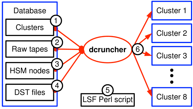
The dcruncher script runs through the following steps (see Figure 5):
-
1.
Check for free dbasf clusters (fastest first).
-
2.
Check for available unprocessed raw tape (depending on cluster type: see speed optimization below).
-
3.
Find location for output file on HSM.
-
4.
Insert corresponding entry in mdst files table.
-
5.
Write Perl script job to submit to LSF batch queue.
-
6.
Send job to relevant cluster (the script job is run on the tape server of the cluster).
-
7.
Wait 5 minutes and restart the loop.
4.3 Speed Optimization
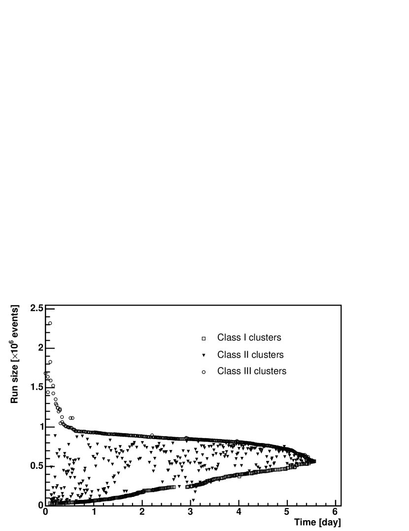
The number of events in each run greatly varies, depending on the operation condition. In order to optimize the allocation of computing power, faster clusters process the largest runs, and slower clusters process the smallest runs. The total process time is indeed roughly proportional to the run size. This simple algorithm is illustrated on Figure 6: the largest runs are processed by class III clusters, while shortest runs are processed by class I clusters. The number of events in runs processed by class II clusters is randomly distributed between these two extrema, because these clusters simply process runs sequentially.
5 PERFORMANCE
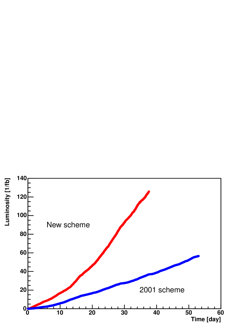
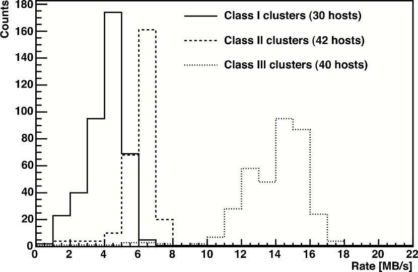
The task of the new scheme was to complete the processing of all the data accumulated from autumn 2003 to summer 2004 (120 TB) before the summer physics conferences. It started running on May 18, 2004 and finished processing on July 12 (56 days in total). It has been actually running for 39 days (delays were mainly due to calibration and updating of the database). 3.3 billion events were processed in 3408 jobs, with a total output size of 40 TB. The average output rate was 3.2/fb/day (37 MB/s), with a peak of 5.1/fb/day (60 MB/s) for 7 consecutive days. In comparison, the previous processing scheme reached an average output rate of 1.1/fb/day (see Figure 7). This older scheme used a slightly different version of dbasf on about half of the computing power. The output rate per cluster class is shown in Figure 8.
5.1 Failures and limitations
During the 39 days of processing, a total of 0.7% of the jobs failed due to an error related to dbasf. The break-down of the errors is shown in Table 2.
| Inter-process communication | 0.2% |
|---|---|
| Database access | 0.1% |
| Tape drives | |
| Network | 0.3% |
| Total | 0.7% |
In addition, a number of limitations to the processing speed have been observed:
Database access is one of the main issues, since processing makes heavy use of the database, in particular at the start of a job. Using more dedicated servers will solve this issue.
The limited CPU power of tape servers which distribute the data the dbasf clusters was identified as the present bottleneck. Faster tape servers will be used in the future.
The network bandwidth between the input server and basf nodes may eventually limit the processing power. This does not seem to be a major issue in the near future.
None of these limitations, however, seriously hampered the processing speed.
6 CONCLUSION
The new offline processing scheme started running on May 18, 2004. In 39 days of stable running, it successfully processed the 3 billion events collected by KEKB with a maximum rate of 5/fb/day, 5 times faster than the data acquisition and the previous scheme. With the expected increase of the KEKB luminosity, however, the DST processing will face further challenges…Room for improvement of this scheme still remains.
References
- [1] A. Abashian et al., Nucl. Instr. and Meth. A479, 117 (2002).
- [2] S. Kurokawa et al., Nucl. Instr. and Meth. A499, 1 (2003).
- [3] R. Itoh, “Experience with Real Time Event Reconstruction Farm for Belle Experiment”, Contribution 209, CHEP’04.
- [4] N. Katayama, “New compact hierarchical mass storage system at Belle”, Contribution 211, CHEP’04.
- [5] http://www.postgresql.org/
- [6] Platform Computing – http://www.platform.com/
- [7] http://www.redhat.com/
- [8] http://www.sun.com/software/solaris/