Anomalous absorption of light by a nanoparticle and bistability in the presence of resonant fluorescent atom

Abstract

Absorption of light by a nanoparticle in the presence of resonant atom and fluorescence of the latter are theoretically investigated. It is shown, that absorption of light by a nanoparticle can be increased by several orders because of presence of atom. It is established, that optical bistability in such system is possible.

PACS numbers: 42.50.Ct, 12.20.-m, 42.60.Da, 42.50.Lc, 42.50.Pq, 42.50.Nn

1 Introduction

The cross-section of light adsorption by an isolated spherical nanoparticle imbedded in a host medium and which radius $a$ is essentially smaller then light wavelength $\lambda$ in the medium ($a/\lambda\ll 1$) is given by the classical formula [1]

$${\sigma}_{p}=24\pi\frac{a}{\lambda}\frac{\epsilon^{\prime\prime}}{|\epsilon+2|^{2}}S\,,$$ (1)

where ${S}=\pi a^{2}$, ${\epsilon}\equiv\varepsilon_{p}/\varepsilon_{h}=\epsilon^{\prime}+i\epsilon^{\prime\prime}$ is the relative complex dielectric function of the nanoparticle, $\varepsilon_{h}$ and $\varepsilon_{p}$ are dielectric functions of the nonabsorbing host medium and nanoparticle respectively.

As a rule, ${\sigma}_{p}$ is smaller then geometrical cross-section of the nanoparticle $S$. On the other hand, it is well known that the cross-section of resonant atom-light interaction is considerably larger:

$${\sigma}_{a}=\frac{1}{2\pi}\frac{\mathstrut{\gamma_{0h}}}{\gamma}{\lambda}^{2}\,,$$ (2)

where $\gamma_{0h}$ and $\gamma$ are the radiation and the total width of the resonant transition of an atom imbedded in a host medium. Note that $\gamma_{0h}$ is expressed in terms of free-space spontaneous emission rate $2\gamma_{0}$ as $\gamma_{0h}\equiv(\varepsilon_{h})^{1/2}|(\varepsilon_{h}+2)/3|\gamma_{0}$ (see, e.g., [2, 3]).

As a rule, ${\sigma}_{p}\ll{\sigma}_{a}$ (see Fig. 1).

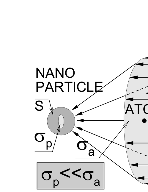
Figure 1: Atomic lens.

The aim of the paper is clarification of the probability of cascade energy transfer from light to an atom and then to a nanoparticle [4], and investigation of atomic fluorescence in this conditions.

2 Oscillating classical dipole

Let us consider an auxiliary problem connected with atomic excitation transfer to a nanoparticle, the particle absorption of the electric field energy of classical dipole ${\mathrm{\mathbf{d}}}\equiv d\{\sin(\psi),0,\cos(\psi)\}$ which oscillates with frequency $\omega$ and is at a distance $\mathrm{\mathbf{R}}$ from the nanoparticle center. The power $Q_{c}$ absorbed by the nanoparticle can be represented in the form

$$Q_{c}=-\overline{\dot{\mathrm{\mathbf{d}}}(\mathrm{\mathbf{R}})\,\delta\mathrm{\mathbf{E}}(\mathrm{\mathbf{R}})}\,,$$ (3)

where $\delta\mathrm{\mathbf{E}}(\mathrm{\mathbf{R}})$ is the ‘image field’ of the dipole, and overline denotes time averaging over the time that is considerably greater than period of light wave. Since $\delta\mathrm{\mathbf{E}}$ depends linearly on $\mathrm{\mathbf{d}}$, the absorbed power $Q_{c}$ can be rewritten as

$$Q_{c}=2\omega\mathop{\mathrm{Im}}\nolimits\left[\sum_{\alpha,\beta}G_{\alpha\beta}(\mathrm{\mathbf{R}},\mathrm{\mathbf{R}};\omega){\mathrm{\mathbf{d}}}_{\beta}{\mathrm{\mathbf{d}}}_{\alpha}\right]\,,$$ (4)

where $G_{\alpha\beta}(\mathrm{\mathbf{R}},\mathrm{\mathbf{R}};\omega)$ is the field susceptibility (or tensor-valued Green function):

$$\delta\mathrm{\mathbf{E}}_{\alpha}(\mathrm{\mathbf{r}},\omega)=\sum_{\beta}G_{\alpha\beta}(\mathrm{\mathbf{r}},\mathrm{\mathbf{r}}^{\prime};\omega){\mathrm{\mathbf{d}}}_{\beta}(\mathrm{\mathbf{r}}^{\prime},\omega)\,.$$ (5)

2.1 Field susceptibility

In the near zone ($R\ll\lambda$) the ‘image field’ of the dipole (and, consequently, $G$) can be found by solving electrostatic Laplace equation. One can start with the scalar potential of a single charge $e$ located on the axis $Z$ at the distance $R$ from the center of the particle [5]):

$$\varphi_{e}(\mathrm{\mathbf{r,R}})=-\frac{e}{a}\sum_{n=0}^{\infty}{\frac{(\epsilon-1)n}{(\epsilon+1)n+1}\,P_{n}\left(\cos(\theta)\right)\left(\frac{a^{2}}{rR}\right)^{n+1}},$$ (6)

where $P_{n}(\cos(\theta))$ is the Legendre polynom and $\theta$ is an elevation angle of the vector $\mathrm{\mathbf{r}}$.

The potential of the point-like dipole $\mathrm{\mathbf{d}}$ located on the axis $Z$ at the distance $R$ from the center of the particle is the sum of potentials (6) caused to nearly situated charges $e$ and $-e$

$$\varphi(\mathrm{\mathbf{r,R}})=\frac{d}{aR}\sum_{n=0}^{\infty}\frac{(\epsilon-1)n}{(\epsilon+1)n+1}\,\bigg{[}(n+1)\cos(\psi)P_{n}\left(\cos(\theta)\right)$$

$$\phantom{\varphi(\mathrm{\mathbf{r,R}})}\left.-\sin(\psi)\sin(\theta)\cos(\phi)\frac{dP_{n}\left(\cos(\theta)\right)}{d\cos(\theta)}\right]\left(\frac{a^{2}}{rR}\right)^{n+1},$$ (7)

where $\phi$ is an azimuth angle of the vector $\mathrm{\mathbf{r}}$.

So, the ‘image field’ and $G$ are found from (2.1) and represented as a series (see, for example, [6]). This series diverges when $R\to a$, so that the higher terms start play the major part in it. Fortunately, one possible to rewrite it in a reasonable way, so that the field susceptibility tensor can be expressed in the form

$$G_{zz}(\mathrm{\mathbf{R}})={\frac{\epsilon-1}{\epsilon+1}\,\frac{\mu^{3}}{\varepsilon_{h}R^{3}}}\left[{\frac{2}{{\varrho}^{3}}}{\,+\frac{1}{{\varrho}^{2}{\rho}}+\frac{1}{{\varrho}{\rho}^{2}}}{-\frac{{\epsilon}^{-1}}{{\rho}^{3}}\,\frac{\epsilon+1}{\epsilon+2}\,F\left(\begin{array}[]{c}{1,1+\nu}\\ {2+\nu}\end{array}\Biggr{|}{\rho}^{-2}\right)}\right],$$ (10)

$$G_{xx}(\mathrm{\mathbf{R}})={\frac{1}{2}\,\frac{\epsilon-1}{\epsilon+1}\,\frac{\mu^{3}}{\varepsilon_{h}R^{3}}}\left[{\frac{2}{{\varrho}^{3}}}{\,-\frac{{\epsilon}^{-1}}{{\varrho}^{2}{\rho}}-\frac{{\epsilon}^{-1}}{\varrho{\rho}^{2}}}{+\frac{{\epsilon}^{-2}}{{\rho}^{3}}\,\frac{\epsilon+1}{\epsilon+2}\,F\left(\begin{array}[]{c}{1,1+\nu}\\ {2+\nu}\end{array}\Biggr{|}{\rho}^{-2}\right)}\right],$$ (13)

where ${\mu}\equiv\epsilon/(\epsilon+1)$, ${\varrho}\equiv{\mu}{\varrho}_{0}$, ${{\varrho}_{0}}\equiv({\rho}-{\rho}^{-1})$, ${\rho}\equiv R/a$, ${\nu}\equiv 1/(\epsilon+1)$, ${\epsilon}\equiv\varepsilon_{p}/\varepsilon_{h}$, $\varepsilon_{p}$ and $\varepsilon_{h}$ are complex dielectric function of the nanoparticle and host surroundings accordingly, $F\left(\begin{array}[]{c}{a,b}\\ c\end{array}\Biggr{|}s\right)$ is hypergeometric function.

Let us concider some limit cases.

• $|\epsilon|\gg 1$ (i.e., ideal conductor)

  $$G_{zz}(\mathrm{\mathbf{R}}) \simeq {\frac{1}{\varepsilon_{h}R^{3}}}\left[{\frac{2}{{\varrho}_{0}^{3}}}{\,+\frac{1}{{\varrho}_{0}^{2}{\rho}}+\frac{1}{{\varrho}_{0}{\rho}^{2}}}\right],$$ (14)

  $$G_{xx}(\mathrm{\mathbf{R}}) \simeq {\frac{1}{\varepsilon_{h}R^{3}{\varrho}_{0}^{3}}}\,.$$ (15)

  As is well known, in this case the ‘image field’ that corresponds to (14) and (15) can be represented by the sum of the fields of the charge ${q_{0}}\equiv ad_{z}/R^{2}$ and $-q_{0}$, and of the dipole ${\mathrm{\mathbf{d}}}_{0}\equiv(a/R)^{3}d\{-\sin(\psi),0,\cos(\psi)\}$ field. The charge -${q_{0}}$ is placed at the particle center; the charge ${q_{0}}$ and dipole ${\mathrm{\mathbf{d}}}_{0}$ are located along $Z$ axis at the distance $a{\varrho}_{0}$ from dipole $\mathrm{\mathbf{d}}$(another words, at distance $a^{2}/R$ from the particle center toward the dipole $\mathrm{\mathbf{d}}$).

Similarly to this limit case, the first three terms in square brackets of the equations (10) and (13) can be interpreted as the sum of the fields of the charges ${q}\equiv\mu^{3}(\epsilon-1)/(\epsilon+1)q_{0}$, $-q$, ${q_{\epsilon}}\equiv-q/\epsilon$, $-q_{\epsilon}$, and of the dipole ${{\mathrm{\mathbf{d}}}_{1}}\equiv\mu^{3}(\epsilon-1)/(\epsilon+1){\mathrm{\mathbf{d}}}_{0}$. Charge ${q}$ and dipole ${{\mathrm{\mathbf{d}}}_{1}}$ are located along $Z$ axis at the distance $R^{\prime}_{1}\equiv a{\varrho}$ from dipole $\mathrm{\mathbf{d}}$, whereas the charge $-q$ is disposed at the distance $R_{1}\equiv a{\rho}\left[\varrho/(\rho/\mu-{\rho}^{-1})\right]^{1/2}$ from dipole $\mathrm{\mathbf{d}}$ along the same $Z$ axis. Charges ${q_{\epsilon}}$ and ${-q_{\epsilon}}$ are located at the distance $R_{1}$ and $R^{\prime}_{1}$ respectively from dipole $\mathrm{\mathbf{d}}$ along $X$ axis (see Fig. 2).

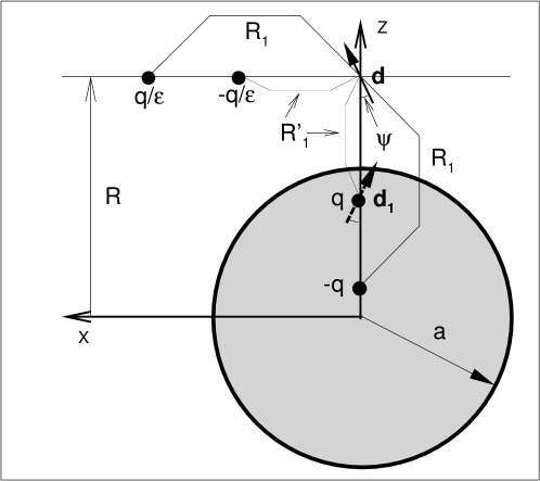
Figure 2: Geometry of the problem.

These terms of the equations (10) and (13) dominate while as $R/a\gtrsim 1$, and $\epsilon$ is far away from the region of the surface multipole resonances that take place when $\mathop{\mathrm{Re}}\nolimits(n+1+\nu)=0$.

• Small distances, $R/a-1\ll 1$ ($\varrho_{0}\simeq 0$)

  $$G_{xx}(\mathrm{\mathbf{R}})\simeq\frac{1}{2}\,G_{zz}(\mathrm{\mathbf{R}})\simeq\frac{\epsilon-1}{\epsilon+1}\,\frac{\mu^{3}}{\varepsilon_{h}R^{3}}\,\frac{1}{{\varrho}^{3}}.$$ (16)

  It is exactly the case of the planar interface.

• Large distances, $R/a\gg 1$ (i.e., $\varrho_{0}\simeq R/a$)

  $$G_{xx}(\mathrm{\mathbf{R}})\simeq\frac{1}{4}\,G_{zz}(\mathrm{\mathbf{R}})\simeq\frac{\epsilon-1}{\epsilon+2}\,\frac{a^{3}}{{\varepsilon}_{h}R^{6}}\,.$$ (17)

  The ‘image field’ corresponding to (17) is given by

  $$\delta\mathrm{\mathbf{E}}(\mathrm{\mathbf{R}})\simeq\frac{\epsilon-1}{\epsilon+2}\,\frac{a^{3}}{{\varepsilon}_{h}R^{6}}\left[3(\mathrm{\mathbf{n}}\mathrm{\mathbf{d}}\,)\mathrm{\mathbf{n}}+\mathrm{\mathbf{d}}\,\right]\,,$$ (18)

  where $\mathrm{\mathbf{n}}$ is the unit vector in the direction from the center of the particle to dipole $\mathrm{\mathbf{d}}$.

Physical interpretation of the formula (18). At large distance the electric field ${\mathrm{\mathbf{E}}_{\mathrm{\mathbf{d}}}}$ of the dipole $\mathrm{\mathbf{d}}$ is homogeneous in the vicinity of the particle. The field of the polarization (or scattered field) $\delta\mathrm{\mathbf{E}}$ of the particle in such homogeneous field $\mathrm{\mathbf{E}}_{\mathrm{\mathbf{d}}}$ at the location of the dipole $\mathrm{\mathbf{d}}$ is given by (see, for example, [1])

$$\delta\mathrm{\mathbf{E}}(\mathrm{\mathbf{R}})=\frac{\epsilon-1}{\epsilon+2}\,\frac{a^{3}}{R^{3}}\left[3(\mathrm{\mathbf{n}}\mathrm{\mathbf{E}}_{\mathrm{\mathbf{d}}})\mathrm{\mathbf{n}}-\mathrm{\mathbf{E}}_{\mathrm{\mathbf{d}}}\right]\,.$$ (19)

In turn, the field $\mathrm{\mathbf{E}}_{\mathrm{\mathbf{d}}}$ in the quasistatic approximation is given, as is well known, by [1]

$$\mathrm{\mathbf{E}}_{\mathrm{\mathbf{d}}}=\frac{1}{{\varepsilon}_{h}R^{3}}\left[3(\mathrm{\mathbf{n}}\mathrm{\mathbf{d}})\mathrm{\mathbf{n}}-\mathrm{\mathbf{d}}\right]\,.$$ (20)

Substituting this expression in (19) we get (18).

3 Quantum consideration

Energy transfer to the nanoparticle from the real atom exited by the light is given by (instead of (4))

$$Q_{c}=2\omega\mathop{\mathrm{Im}}\nolimits\left[\sum_{\alpha,\beta}G_{\alpha\beta}(\mathrm{\mathbf{R}};\omega)\langle\colon\hat{\mathrm{\mathbf{d}}}_{\beta}^{-}\hat{\mathrm{\mathbf{d}}}_{\alpha}^{+}:\rangle\right]\,,$$ (21)

where symbols ‘$\colon\,\colon$’ and ‘$\langle\cdots\rangle$’ denote the normal ordering operator and the quantum averaging respectively. For two-level atom $\hat{\mathrm{\mathbf{d}}}^{+}$ is

$$\hat{\mathrm{\mathbf{d}}}^{+}=\left\{\hat{\mathrm{\mathbf{d}}}^{-}\right\}^{{\dagger}}=\mathrm{\mathbf{d}}_{nm}\exp\left(i\Omega_{0}t\right)\hat{\sigma}_{-}\,,$$ (22)

where $\Omega_{0}\equiv\omega-\omega_{mn}$, $\mathrm{\mathbf{d}}_{mn}$ and $\omega_{mn}$ are matrix element of the dipole moment of the $m-n$ atomic transition and the resonance frequency of this transition, $\hat{\sigma}_{\pm}$ are the raising and lowering Pauli’s operators.

Substituting (22) in (21) results in

$$Q_{c}=2\omega\mathop{\mathrm{Im}}\nolimits\left[\sum_{\alpha,\beta}G_{\alpha\beta}(\mathrm{\mathbf{R}};\omega){\mathrm{\mathbf{d}}_{nm}}_{\beta}{\mathrm{\mathbf{d}}_{mn}}_{\alpha}\right]\rho_{m}\equiv 2\hbar\omega\gamma_{c}\rho_{m}\,,$$ (23)

where $\rho_{m}$ is population of the upper atomic level $m$, and $\gamma_{c}$ is the addition nonradiative broadening of the atomic transition due to energy transfer from the atom to the particle (see below).

4 Density matrix

Density matrix for two-level atom in the vicinity of the nanoparticle obey the follow system of the equations [7]

$$\frac{d\rho}{dt} = -(\gamma-i\Omega)\rho-i{\Omega}_{R}\Delta/2\,,$$ (24)

$$\frac{d\Delta}{dt} = -2\gamma(1+\Delta)-2\mathop{\mathrm{Im}}\nolimits\left[\Omega_{R}{\rho}^{*}\right]\,.$$ (25)

where ${\Delta}\equiv\rho_{m}-\rho_{n}=\langle{\hat{\sigma}}_{3}\rangle$ and ${\rho}\equiv\langle{\hat{\sigma}}_{-}\rangle\exp(i\omega t)$ are the population difference and coherence of combining levels, ${\Omega_{R}}=|\mathrm{\mathbf{E}}\cdot\mathrm{\mathbf{d}}_{mn}|/\hbar$ is Rabi frequency, $\mathrm{\mathbf{E}}$ is an local electric field acting on the atom, ${\Omega}=\Omega_{0}+\nu$, ${\nu}=\mathop{\mathrm{Re}}\nolimits(\Gamma)$, ${\gamma}=\mathop{\mathrm{Im}}\nolimits(\Gamma)$,

$$\Gamma=\frac{1}{\hbar}\,\left[\sum_{\alpha,\beta}(\mathrm{\mathbf{d}}_{mn})_{\alpha}G_{\alpha\beta}^{ex}(\mathrm{\mathbf{R}})(\mathrm{\mathbf{d}}_{mn}^{*})_{\beta}\right]\,.$$ (26)

Here $G^{ex}$ is the exact field susceptibility. Therefore the imaginary part of Eq. (26) as the total decay rate, $\gamma=\gamma_{r}+\gamma_{c}$, describes both radiative decay $\gamma_{r}$ and nonradiative one $\gamma_{c}$.

The field susceptibility, $G$, Eqs. (10)–(13), is the quasistatic approximation of the exact one, $G^{ex}$. Hence, it is responsible for nonradiative decay only. Nevertherless, the radiative part of the decay rate can be found in our case by use of quasistatic solution (2.1). Indeed, the solution represents multipole expansion of the scalar potential induced by dipole $\mathrm{\mathbf{d}}$. In the near zone the dipole part of the induced potential (2.1) is described by its term with $n=1$

$$\varphi^{(1)}(\mathrm{\mathbf{r,R}})=\frac{d}{r^{2}}\,\frac{\epsilon-1}{\epsilon+2}\,\frac{a^{3}}{R^{3}}\,\left[2\cos(\psi)\cos(\theta)-\sin(\psi)\sin(\theta)\cos(\phi)\right]\equiv\frac{{\mathrm{\mathbf{d}}}_{p}\cdot\mathrm{\mathbf{r}}}{r^{3}}\,,$$ (27)

$${\mathrm{\mathbf{d}}}_{p}\equiv d\,\frac{\epsilon-1}{\epsilon+2}\,\frac{a^{3}}{R^{3}}\,\{-\sin(\psi),0,2\cos(\psi)\}.$$ (28)

Dipoles $\mathrm{\mathbf{d}}$ and ${\mathrm{\mathbf{d}}}_{p}$ oscillate in phase due to the inequality $a,R\ll\lambda$. So, the emission probability and intensity of radiation are proportional to the total dipole squared $|\mathrm{\mathbf{d}}$ + ${\mathrm{\mathbf{d}}}_{p}|^{2}$. Hence, the radiative part of the spontaneous decay rate of an atom placed next to a nanoparticle is given by

$${\gamma_{r}}={\gamma_{0h}}\,\left[\left|1-\frac{\epsilon-1}{\epsilon+2}\,\frac{a^{3}}{R^{3}}\right|^{2}\sin^{2}(\psi)+\left|1+2\frac{\epsilon-1}{\epsilon+2}\,\frac{a^{3}}{R^{3}}\right|^{2}\cos^{2}(\psi)\right],$$ (29)

Expression (29) agrees with the radiative part of the spontaneous decay rate calculated without assumption of the quasistatic approximation in the limit $a/\lambda\to 0$ [8].

Steady-state solution of the equations (24), (25) is conveniently expressed by

$$\rho_{m}=\frac{1}{2}\,\frac{{\tilde{\gamma}}^{-2}\xi^{2}g(\tilde{\Omega})\tilde{I}/2}{1+\mathstrut{\tilde{\gamma}}^{-2}\xi^{2}g(\tilde{\Omega})\tilde{I}/2}\,,$$ (30)

where following dimensionless quantities are introduced: the total broadening of the transition ${\tilde{\gamma}}\equiv{\gamma_{r}}/{\gamma_{0h}}+{\gamma_{c}}/{\gamma_{0h}}$

$$\tilde{\gamma} \equiv \left[\left|1-\frac{\epsilon-1}{\epsilon+2}\,\frac{a^{3}}{R^{3}}\right|^{2}\sin^{2}(\psi)+\left|1+2\frac{\epsilon-1}{\epsilon+2}\,\frac{a^{3}}{R^{3}}\right|^{2}\cos^{2}(\psi)\right]$$ (31)

$$+ k^{-3}\mathop{\mathrm{Im}}\nolimits\left[G_{zz}(\mathrm{\mathbf{R}})\cos^{2}(\psi)+G_{xx}(\mathrm{\mathbf{R}})\sin^{2}(\psi)\right]$$

($k$ is the wave vector of the light in the medium, ${\psi}$ is the angle between $\mathrm{\mathbf{R}}$ and $\mathrm{\mathbf{d}}\sim\mathrm{\mathbf{E}}$); local field gain factor ${\xi}\equiv\left|{E}/{E_{0}}\right|$

$$\xi=\left|\left\{\mathrm{\mathbf{e}}_{0}+{\frac{\epsilon-1}{\epsilon+2}\frac{a^{3}}{R^{3}}\left[3(\mathrm{\mathbf{e}}_{0}\cdot\mathrm{\mathbf{n}})\mathrm{\mathbf{n}}-\mathrm{\mathbf{e}}_{0}\right]}\right\}\right|$$ (32)

(${E_{0}}$ and ${\mathrm{\mathbf{e}}_{0}}$ are amplitude and unit polarization vector of the incident light wave); formfactor of the optical transition line ${g(\tilde{\Omega})}/\pi\equiv\pi^{-1}/(1+{\tilde{\Omega}}^{2})$; ${\tilde{\Omega}}\equiv\Omega/(\gamma_{r}+\gamma_{c})$; and intensity of the incident light ${\tilde{I}}\equiv I/I_{s}$, where ${I_{s}}\equiv\hbar\omega\gamma_{0h}/\sigma_{a}$ is saturated intensity of free atom in the medium, ${\sigma_{a}}$ is resonance cross-section (2). The second term in the braces of (32) multiplied by $E_{0}$ is the scattered field of the nanoparticle in the near zone.

5 Efficiency of the cascade energy transfer

Efficiency of the cascade energy transfer ${\eta}\equiv Q_{c}/Q_{p}$ (where ${Q_{p}}=I\sigma_{p}$) can be found by using expressions (1), (23) and (30)

$$\eta\equiv\frac{1}{24\pi}\,\frac{\lambda}{a}\,\frac{\sigma_{a}}{S}\,\frac{|\epsilon+2|^{2}}{\epsilon^{\prime\prime}I}\,\frac{\frac{1}{2}\tilde{\gamma}_{c}{\tilde{\gamma}}^{-2}\xi^{2}g(\tilde{\Omega})\tilde{I}}{1+\frac{1}{2}\mathstrut\tilde{\gamma}^{-2}\xi^{2}g(\tilde{\Omega})\tilde{I}}.$$ (33)

Obvious, efficiency of the cascade energy transfer can rich as much as several orders of magnitude because of multiplication of large values $\lambda/a$, $\sigma_{a}/S$, $|\epsilon+2|^{2}/\epsilon^{\prime\prime}$.

The limit cases

• Large distances, $R/a\gg 1$
  In this case $\tilde{\gamma}\to 1$, $\tilde{\gamma}_{c}\sim R^{-6}$ (see Eqs. (31) and (17)). Hence, Eq. (33) is became

  $$\eta\sim R^{-6}.$$

• Small distances, $R/a-1\ll 1$
  In this conditions $\tilde{\gamma}\approx\tilde{\gamma}_{c}\sim(R/a-a/R)^{-3}$ (see Eqs. (31) and (15)). Assuming in addition $\frac{1}{2}\mathstrut\tilde{\gamma}^{-2}\xi^{2}g(\tilde{\Omega})\tilde{I}\ll 1$, we get from Eq. (33)

  $$\eta\sim(R/a-a/R)^{3}.$$

  This decreasing of $\eta$ is rather unexpected because the probability of the energy transfer from atom to nanoparticle is about 1 in this case. However, atomic resonance cross-section is decreased when $\gamma$ is increased (see Eq.(2)).

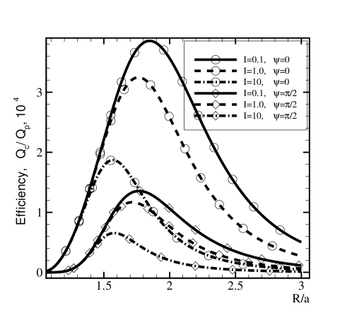
Figure 3: Efficiency of the cascade energy transfer as a function of the dimensionless distance $R/a$ between resonance atom and centre of the nanoparticle. It is supposed that the light frequency is tuned in to the resonance atomic frequency at any distance. Calculations are made for a silver nanoparticle ($\varepsilon_{p}=-15.37+i0.231$, $\lambda=6328$ nm)

So, the efficiency is decreased both for large and small distances between atom and particle. Therefore, it achieves a maximum at an intermediate $R\gtrsim a$. Fig. 3 shows efficiency of the cascade energy transfer $\eta$ versus $R/a$ in the assumption of the exact resonance at any $R/a$.

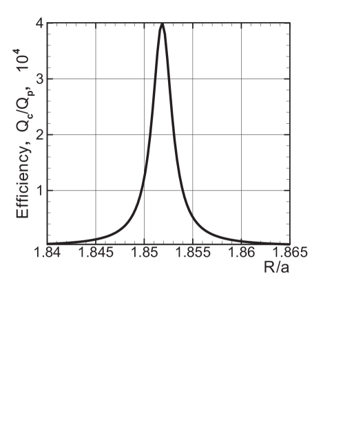
Figure 4: The same as in Fig. 3, but for fixed light frequency $\tilde{\Omega}\equiv\Omega/\gamma_{0}=-410$.

On the other hand, figure Fig. 4 demonstrates very sharp resonance dependence of $\eta$ as a function of $R/a$ when the frequency of the light wave is fixed.

This sharply outlined resonance can be used to determine location of an atom regarding the surface with subnanometer precision.

6 Fluorescence

As it is known, the intensity of fluorescence $I_{f}$ is proportional to $\gamma_{r}\rho_{m}$. Using Eqs. (29)–(30), intensity of fluorescence can be written by

$$I_{f}=I_{0}\,\frac{\frac{1}{2}\tilde{\gamma}_{r}{\tilde{\gamma}}^{-2}\xi^{2}g(\tilde{\Omega})\tilde{I}}{1+\frac{1}{2}\mathstrut\tilde{\gamma}^{-2}\xi^{2}g(\tilde{\Omega})\tilde{I}}.$$ (34)

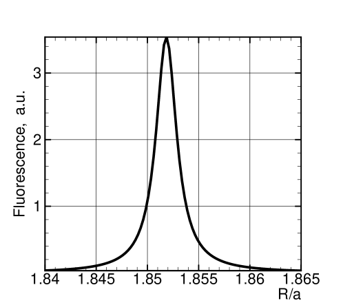
Figure 5: Intensity of fluorescence, a.u., as a function of $R/a$. Conditions are the same as in Fig. 4.

Fig. 5 shows the intensity of fluorescence, a.u., as a function of $R/a$. Conditions are the same as in Fig. 4.

7 Heating of the particle

Basic approaches and approximations

• Steady-state approximation

• Uniform temperature ${T_{p}}$ inside the particle

• Laplace’s equation $\Delta T_{h}=0$ for the temperature of the host medium

• Energy balance equation
  $Q_{c}+Q_{p}=\varkappa\int\mathrm{\mathbf{\nabla}}T_{h}\,d\mathrm{\mathbf{S}}$
  where ${\varkappa}$ is thermal conductivity of surroundings

• Linear temperature dependence of $\varepsilon_{p}^{\prime\prime}$:
  $\varepsilon_{p}^{\prime\prime}=\varepsilon_{p0}^{\prime\prime}+{\alpha}(T_{p}-T_{0})$

• $|\varepsilon_{p}^{\prime\prime}/(\varepsilon_{p}^{\prime}+\varepsilon_{h}^{\prime})|$, $|\varepsilon_{h}/\varepsilon_{p}^{\prime}|\ll 1$

Solution of the Laplace’s equations is

$$T_{h}(r)=T_{0}+\frac{a}{r}(T_{p}-T_{0})\,.$$ (35)

It gives a linear temperature dependence of heat removing from the particle

$$Q_{T}=Q_{c}+Q_{p}=4\pi\varkappa a(T_{p}-T_{0})\,.$$ (36)

Substituting (1) and (33) in this equation results in following cubic equation with respect to the relative increase of the image part of the dielectric function of the nanoparticle ${z}\equiv\delta\varepsilon_{p}^{\prime\prime}/\varepsilon_{p0}^{\prime\prime}$:

$$(x-y-1)z^{3}+\left[3(x-y)-2]+[3(x-y)-1+(x-1)f\right]z+xf+x-y=0\,,$$ (37)

where the following dimensionless quantities are introduced: ${f}\equiv\frac{1}{2}\mathstrut\tilde{\gamma}^{-2}\xi^{2}g(\tilde{\Omega})\tilde{I}$ is saturation factor, ${x}\equiv(N_{p}+1)z/N$, ${y}\equiv\Delta z/N$, ${z/N}\equiv\left[{\hbar\omega_{mn}\gamma_{c}}/({{4\pi a\varkappa}})\right]\left[{\alpha}/{\varepsilon_{p0}^{\prime\prime}}\right]$, ${N_{p0}}\equiv Q_{p0}/(\hbar\omega_{mn}\gamma_{c})$ and ${N}\equiv Q_{T}/(\hbar\omega_{mn}\gamma_{c})$ are the number of photons absorbed by the nanoparticle during the time $\gamma_{c}^{-1}$ directly from the light wave and the total one respectively.

As well known, the qubic equation (37) may have 3 solution at some parameters. Therefore, $z$ may exhibit bistable behaviour. In the Fig. 6 it is shown the regions of such bistability.

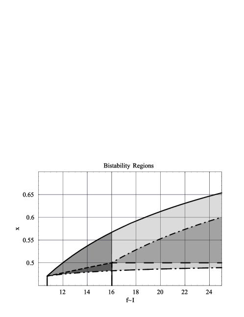
Figure 6: Bistability regions of the the relative increase of the image part of the dielectric function of the nanoparticle ${z}=\delta\varepsilon_{p}^{\prime\prime}/\varepsilon_{p0}^{\prime\prime}$. The range of values of parameter ${y}=\Delta z/N$ which depends on ${x}=(N_{p}+1)z/N$ and saturation factor ${f}=\frac{1}{2}\tilde{\gamma}^{-2}\xi^{2}g(\tilde{\Omega})\tilde{I}$ is different in each domain (${N_{p0}}\equiv Q_{p0}/(\hbar\omega_{mn}\gamma_{c})$ and ${N}\equiv Q_{T}/(\hbar\omega_{mn}\gamma_{c})$ are the number of photons absorbed by the nanoparticle during the time $\gamma_{c}^{-1}$ directly from the light wave and the total one respectively.). However, parameter $y$ is always negative in all domains of bistability.

8 Conclusions

• Cascade energy transfer efficiency can rich as mach as several order of magnitude ($10^{3}-10^{5}$)

• Efficiency is drastically decreased at both large and small distances between atom and nanoparticle surface

• For constant light frequency the efficiency as sharply as resonance depends from the distance between atom and nanoparticle

• This sharp dependence can be used to determine the atom position near the surface

• Bistability may take place when the population difference and the relative growth of the image part of the particle dielectric function have the opposite signs.

The work was supported by RFBR, grant # 02-02-17885.

References

- [1] L. Landau and E. Lifshitz, Electrodynamics of continuous media. Pergamon, Oxford, 1960.
- [2] S. M. Barnett, B. Huttner, and R. Loudon, “Spontaneous emission in absorbing dielectric media,” Phys. Rev. Lett. 68 (1992) 3698–3701.
- [3] S. M. Barnett, B. Huttner, R. Loudon, and R. Matloob, “Decay of excited atoms in absorbing dielectrics,” J. Phys. B: At. Mol. Phys. 29 (1996) 3763 –3781.
- [4] G. N. Nikolaev, “Induced resonant absorption of electrovagnetic waves by a microparticle,” Phys. Lett. A 140 (1989) 425–428.
- [5] J. A. Stratton, Electromagnetic Theory. McGrow-Hill, New York, 1941.
- [6] V. V. Klimov, M. Ducloy, and V. S. Letokhov, “Radiative frequency shift and linewidth of an atom dipole in the vicinity of a dielectric microsphere,” J. Modern Opt. 43 (1996) 2251–2267.
- [7] G. N. Nikolaev, “Optical bistability of atoms near a material object,” Sov. Phys. JETP Lett. 52 (1990) 425–428.
- [8] V. V. Klimov, M. Ducloy, and V. S. Letokhov, “Spontaneous emission of an atom in the presence of nanobodies,” Quantum Electron. 31 (2001) 569–586.