A new parallel strategy for two-dimensional incompressible flow simulations using pseudo-spectral methods

Abstract

A novel parallel technique for Fourier-Galerkin pseudo-spectral methods with applications to two-dimensional Navier-Stokes equations and inviscid Boussinesq approximation equations is presented. It takes the advantage of the programming structure of the phase-shift de-aliased scheme for pseudo-spectral codes, and combines the task-distribution strategy [Yin, Clercx and Montgomery, Comput. Fluids, 33, 509 (2004)] and parallelized Fast Fourier Transform scheme. The performances of the resulting MPI Fortran90 codes with the new procedure on SGI 3800 are reported. For fixed resolution of the same problem, the peak speed of the new scheme can be twice as fast as the old parallel methods. The parallelized codes are used to solve some challenging numerical problems governed by the Navier-Stokes equations and the Boussinesq equations. Two interesting physical problems, namely, the double-valued $\omega$-$\psi$ structure in two-dimensional decaying turbulence and the collapse of the bubble cap in the Boussinesq simulation, are solved by using the proposed parallel algorithms.

, ,

1 Introduction

The pseudo-spectral method has been very popular in the research of highly accurate numerical simulations since the pioneer work of Orszag and Patterson  [2, 3]. For smooth solutions, the convergence order of the spectral methods is higher than any algebraic power of mesh size. For a comparable error on the uniform mesh, a much finer mesh is required for finite difference or finite element methods. This is one of the reasons that the spectral method has been widely used in spite of the prosperous development of adaptive grid methods. Some comprehensive overviews of the various applications of spectral methods in fluid dynamics can be found in  [4, 5]. With the fast development of supercomputers, more and more efforts have been devoted to parallelizing spectral methods. For challenging simulation problems such as turbulence research, many new interesting phenomena are discovered using large scale parallel computations ($512^{3}-4096^{3}$) (e.g. see  [6, 7], and a review paper  [8]). The parallel schemes based on spectral methods have also been intensively investigated over the last decade—mainly for three-dimensional (3D) problems  [9, 10, 11, 12, 13, 14, 15, 16]. The main computation time for spectral methods is concentrated in the part of the Fast Fourier Transform (FFT), around which the 3D parallel schemes are constructed. In the following, we will denote this parallel FFT procedure as PFFT.

For high dimensional FFT, the transpose-split method can provide very high parallel efficiency, so most commonly used 3D parallel schemes employ this kind of parallel FFT  [9, 10, 11, 12, 13]. Iovieno et al.  [14] combined the transpose-split method and de-aliased procedure in pseudo-spectral codes together to yield high parallel efficiency. Based on the three time-evolution equations of the 3D Navier-Stokes (NS) equations, Basu adopted a parallel scheme which can only be used on a 3-processor computer  [15]. Ling et al.  [16] try to parallel the 3D code by combining the 3-CPU method and the PFFT scheme, and a comparison showed that the combined scheme is always slower than PFFT.

In contrast to the world-wide efforts in 3D parallelization, rather limited efforts have been devoted to parallelizing the two-dimensional simulations  [17, 1]. It is quite common to treat the 2D parallel spectral code as a simplified version of the 3D codes, which are very efficient only in 3D cases (PFFT). As a result, the ratio of the communication time to the computation time in those 2D parallel codes is relatively large, and the parallel efficiency is much lower compared with the corresponding 3D codes (see a short discussion about this topic in  [1]).

To minimize the relative long communication time, Yin et al.  [1] propose a parallel task distribution scheme (PTD) in the 2D pseudo-spectral NS code. Although this scheme is very easy to implement with a good parallel efficiency, it has the limitation that the code can only use 2, 4, and 6 processors to do the calculation.

In this paper, we will parallel the 2D spectral codes by combining the PTD and PFFT schemes. The new strategy overcomes the shortcomings of the former schemes and shows a significant improvement in parallel efficiency. In the following, we will denote this combined strategy as PTF scheme (parallelization through task distribution and FFT).

The paper is organized as follows. In Section 2, the PTF scheme is applied to solve the 2D NS equation; the benchmark of the parallel code on SGI 3800 is presented. We also show several long-time numerical simulations with high resolutions, which reveal some interesting physical phenomena of 2D decaying turbulence  [18, 19]. Of course, PTF plays an important role in those long-time runs. In section 3, the new scheme is applied to solve the 2D inviscid Boussinesq equations. A challenging numerical problem, which is studied previously in  [20, 21, 22], is investigated with three kinds of resolutions ($1024^{2}$, $2048^{2}$, and $4096^{2}$). Finally, a summary of this work is given, where the prospects of the new scheme are also discussed.

2 Parallel 2D pseudo-spectral code for the NS equations

The study of the 2D turbulence distinguishes itself from the 3D turbulence due to its unique phenomena such as inverse energy cascade and self-organization. In the past few decades, a particular kind of statistical mechanics [23] has been widely adopted to study the 2D freely decaying turbulence (see  [18] and references therein).

As a powerful tool, direct numerical simulations (DNS) provide some useful theory check and inspire the deeper thoughts of the statistical theory (e.g. see  [18, 19]). Those simulations normally need to last as long as 100-1000 eddy turnover times before final states of the 2D decaying turbulence are reached. This means that the total calculations of this kind of 2D DNS, although has a smaller array, are more or less the same as those of some short-term 3D DNS. For example, 20 time steps of a 2D DNS with the resolution of $1024^{2}$ will take roughly the same CPU time as one time step of a 3D DNS on a grid of $256^{3}$ on the same computer. On the other hand, because the time evolution loop is impossible to be parallelized, the parallel procedure within one time step becomes essential to improve the performance of a 2D DNS code.

On modern supercomputers, the total CPU time involved in the 2D DNS is not as enormous as that of the 3D DNS if the grid points are the same in each dimension. The peak performance of the parallel code, which is indicated by the shortest wall clock time regardless of the number of CPUs used, becomes more important in 2D DNS. In our research, we would like to get our 2D DNS results in 3 days using 32 CPUs rather than wait for a week using 8 CPUs, although we only achieve a speedup of 2.33 by the fourfold processors. As will be seen later in this paper, the significant improvement of the peak speed is a big advantage of the PTF scheme.

2.1 The governing equations and pseudo-spectral methods

The 2D incompressible NS equation are usually written as

$$\frac{\partial{\rm{\bf u}}}{\partial t}+{\rm{\bf u}}\cdot\nabla{\rm{\bf u}}=-\nabla p+\nu\Delta{\rm{\bf u}},$$ (1)

$$\nabla\cdot{\rm{\bf u}}=0,$$ (2)

where ${\rm{\bf u}}=(\mbox{u,v})$ is the velocity, $p$ is the pressure, and $\nu$ is the kinematic viscosity. Using the vorticity ${\rm{\bf\omega}}=(0,0,\omega)=\nabla\times{\rm{\bf u}}$ and stream function $\psi$, Eq. (1) and (2) can be rewritten as:

$$\frac{\partial\omega}{\partial t}+{\rm{\bf u}}\cdot\nabla\omega=\nu\Delta\omega,$$ (3)

$$\Delta\psi=-\omega.$$ (4)

The stream function is related to velocity by $\mbox{u}={\partial\psi}\mathord{\left/{\vphantom{{\partial\psi}{\partial y}}}\right.\kern-1.2pt}{\partial y}$ and $\mbox{v}=-{\partial\psi}\mathord{\left/{\vphantom{{\partial\psi}{\partial x}}}\right.\kern-1.2pt}{\partial x}$. In the conservative form, Eq. (3) becomes

$$\frac{\partial\omega}{\partial t}+\nabla\cdot(\omega{\kern 1.0pt}{\rm{\bf u}})=\nu\Delta\omega.$$ (5)

We adopted ABCN scheme to carry out the time integration, which discretizes the nonlinear term $\nabla\cdot(\omega{\kern 1.0pt}{\rm{\bf u}})$ with a 2^nd order Adams-Bashforth scheme and the dissipation term $\nu\Delta\omega$ with the Crank-Nicolson scheme. The particular time-stepping used is independent of the parallelization. More accurate schemes, such as 4^th order Runge-Kutta, could also be used.

When Eqs. (4) and (5) are solved by Galerkin pseudo-spectral methods, the Fourier coefficients of $\omega$ are evaluated at each time step. The nonlinear term $\nabla\cdot(\omega{\kern 1.0pt}{\rm{\bf u}})$ is obtained by being transferred back and from the physical space with FFTs; in the meantime, the de-aliasing procedure has to be adopted to remove the aliasing error. There are two kinds of de-aliasing techniques available: padding-truncation and phase-shifts  [4]. The FFT we used requires the dimension size to be the power of 2, which is faster than those FFTs that has prime factors other than 2. The costs of two de-aliasing techniques are the same as that for our FFTs. Therefore, in this paper we use the phase-shifts, which reserves more high wave numbers information than that for padding-truncation.

Table 1: Ten FFTs need to be calculated in each time step of NS spectral solver.

	A	B	C	D
1	$\hat{\mbox{u}}\to\mbox{u}$	$\hat{\mbox{v}}\to\mbox{v}$	$\hat{\mbox{U}}\to\mbox{U}$	$\hat{\mbox{V}}\to\mbox{V}$
2	$\hskip 50.58878pt\hat{\omega}\to\omega$		$\hskip 50.58878pt\hat{\Omega}\to\Omega$
3	$\mbox{u}\omega\to\widehat{\left({\mbox{u}\omega}\right)}$	$\mbox{v}\omega\to\widehat{\left({\mbox{v}\omega}\right)}$	$\mbox{U}\Omega\to\widehat{\left({\mbox{U}\Omega}\right)}$	$\mbox{V}\Omega\to\widehat{\left({\mbox{V}\Omega}\right)}$

Table 1 shows the ten FFTs needed to solve Eqs. (4) and (5) in each time step. The expression with a hat (e.g. $\hat{u},\;\widehat{(\mbox{U}\Omega)}$) is the spectral space value of the corresponding physical value without hat ($u,\;\left({\mbox{U$\Omega$ }}\right)$, etc.). The capital letters denote the phase-shift values of the corresponding lower case variables. For example, in a simulation with $M^{2}$ resolution:

$$\Omega_{\rm{\bf j}}=\sum\limits_{\rm{\bf k}}{\hat{\omega}_{k}e^{i{\rm{\bf k}}\cdot\left({{\rm{\bf x}}_{\rm{\bf j}}+\delta}\right)}},$$

where, ${\rm{\bf j}}$ indicates the grid point, ${\rm{\bf k}}$ is the wave number, ${\rm{\bf x}}=(x,y)$, and $\delta=\left({\pi/M,\pi/M}\right)$. Each arrow in Table 1 indicated one 2D FFT, and the four FFTs in the third row should be calculated after the six FFTs in the first two rows (see Fig.3 of  [1] for an even clear picture).

It is worth to mention that the pseudo-spectral method needs to evaluate twelve FFTs for the non-conservative form (Eqs. (3) and (4)), since the two FFTs in the 2^nd row of Table 1 are replaced by four FFTs to transfer $\widehat{\left({{\partial\omega}\mathord{\left/{\vphantom{{\partial\omega}{\partial x}}}\right.\kern-1.2pt}{\partial x}}\right)}$, $\widehat{\left({{\partial\omega}\mathord{\left/{\vphantom{{\partial\omega}{\partial y}}}\right.\kern-1.2pt}{\partial y}}\right)}$, and their phase-shift counterparts to physical space. (Of course, the FFTs in the 3^rd row need to be changed correspondingly although no more FFT is needed.) Hence, it is a natural choice to use the conservative formulation when we use PFFT scheme to parallel the 2D NS code.

In the following subsection, we will give a brief discussion for the PFFT scheme. We will also introduce some symbols and analyzing tools that will be used throughout the paper.

2.2 A brief discussion for the PFFT scheme

The PFFT scheme calculates the ten parallelized FFTs one after another according to certain sequence mentioned in the previous subsection. In our case, the parallelized FFT is the widely-adopted transpose-split parallel scheme, which computes one dimensional (1D) FFT in each direction combined with the data transfer between CPUs and matrix transpose  [10, 24].

It is observed that the research on parallel FFT is a fast developed field (e.g. see  [25, 26, 27, 28], or a relatively complete review in  [29]). It is difficult to rank the available FFTs, since there are so many different versions of FFTs, different parallel schemes for the FFTs, and different parallel computers to implement them. There is an argument that the transpose-split scheme is no longer the clear winner (chapter 23 of Ref  [29]) because it can not avoid the data communication while using 1D FFT in two directions. In this paper, we will not devote our efforts to parallel FFT (simply use the most popular transpose-split), instead, we will try to find other methods to improve the parallel efficiency. Our parallel scheme will be even faster if a faster parallel FFT is adopted.

The total time ($T_{sum}$) for each processor is the sum of the computation time ($T_{comp}$) and the communication time ($T_{comm}$):

$$T_{sum}=T_{comp}+T_{comm}.$$ (6)

In the case of PFFT, the 2D NS equations need to calculate ten FFTs, which makes the major part of the computations. If the resolution of the simulation is $M^{2}$, then

$$T_{comp}=10\times\frac{t_{FFT}}{p}=\frac{10}{p}\times\left({M^{2}\log_{2}\left({M^{2}}\right)\;t_{c}}\right),$$ (7)

where, $p$ is the total number of processors, $t_{FFT}$ is the time that requires by one processor to compute one FFT, and $t_{c}$ is CPU time of one FFT in a single processor times a factor (the factor is 5 in the case of full complex FFT, and 5/2 for real-complex FFT)  [4]. For each FFT, one processor needs to send ($p-1$) blocks of data to other ($p-1$) processors, and receives the same amount of data from all other processors. The size of each block is $M^{2}/p^{2}$, so

$$T_{comm}=2\times\left({(p-1)\times\frac{M^{2}}{p^{2}}\times t_{sendrec}+(p-1)\times t_{delay}}\right)\times 10,$$ (8)

where, $t_{sendrec}$ is the time to transmit a word between processors, and $t_{delay}$ is the latency time for a message passing. For the convenience of the analysis later, it is useful to divide $T_{comm}$ into two parts – transmission time ($T_{sendrec}$) and latency time ($T_{delay}$):

$$T_{sendrec} = 2\times\left({(p-1)\times\frac{M^{2}}{p^{2}}\times t_{sendrec}}\right)\times 10,$$ (9)

$$T_{delay} = 2\times\left({(p-1)\times t_{delay}}\right)\times 10.$$ (10)

Hence, according to our analytical model, the total time for one time step on one processor is:

$$T_{sum} = (20p-20)\times\frac{M^{2}}{p^{2}}\times t_{sendrec}+(20p-20)\times t_{delay}$$ (11)

$$\quad+\frac{10}{p}\times\left({M^{2}\log_{2}\left({M^{2}}\right)\;t_{c}}\right).$$

In fact, the values of $t_{c}$ is smaller for larger CPU numbers because of the cache effect (see the discussion later in this subsection), while $t_{sendrec}$ and $t_{delay}$ are almost constant for a given parallel computer. Here, we are only trying to give an estimated analysis and treat $t_{sendrec}$, $t_{delay}$, and $t_{c}$ as constant; accurate timing work will be the speedup plot resulting from the wall clock time (see, e.g., Fig. 1, the similar approach is also adopted in  [13]).

For many parallel systems, $t_{delay}$ is much larger than $t_{sendrec}$ (sometimes a factor of 1000  [30]), so $T_{delay}$ is a nontrivial part of $T_{sum}$, especially when $M^{2}$ is small. According to Eq. (11), if we use more processors in the simulation, $T_{delay}$ will become larger while the rest part ($T_{sendrec}+T_{comp}$) will be smaller. Eventually, $T_{delay}$ will become the dominating part of $T_{sum}$, which affects the parallel efficiency of the PFFT scheme. In the case of the 2D DNS, this phenomenon is seen in relatively small CPU numbers, because $T_{sendrec}+T_{comp}$ is not very large. In the 3D DNS with high resolutions ($512^{3}$ or higher), $T_{delay}$ will take a very small portion in $T_{sum}$ except for very large $p$. This is the main difference between the 2D and 3D problems.

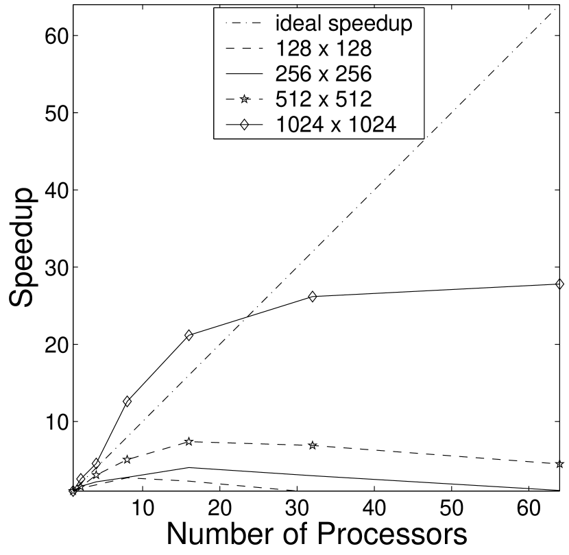
Figure 1: The speedup of 2D Navier-Stokes code with PFFT scheme (or “1-n” scheme).

Fig. 1 shows the speedup of PFFT on different resolutions. The speedup factor is the wall clock time of serial code divided by that of the parallel code in the same resolution. For the resolution of $128^{2}$, the run with eight processors has the top speed. If the CPU number is larger than eight, the speed of the code drops down, and the parallel code with 32 or 64 processors is even slower than the serial code. For resolutions of $256^{2}$ and $512^{2}$, 16 CPUs give the best performance, while 32 and 64 CPUs lead to worse performance. For $1024^{2}$, the fastest run is the one with the maximum available CPUs. (The SGI 3800 in our laboratory is a 64-nodes system; we can not test the cases with more than 64 processors.) We can predict from the tendency of the curve (or, Eq. (11)) that the speedup will also drop down for the $1024^{2}$ run with 128 or more processors.

One may notice that the super-linear speedup for runs with $1024^{2}$ resolution: in the case of 16 CPUs, a speedup of 21 is observed. The super-linear speedup is due to the so-called cache effect. In the architecture of modern computers, caches, which can be viewed as a smaller and faster memory, are widely used to increase the computer performance. For the PFFT NS simulation with fixed $M^{2}$, the more CPUs are involved, the higher hit rate of cache will be obtained because the code exhibits sufficient data locality in its memory accesses. Hence, the unit calculation finished on one CPU in the PFFT code is faster than one CPU with the serial codes, that is, $t_{c}$ is smaller. The behavior of the cache memory is very hard to predict, because modern computer architectures have very complex internal organizations: different levels of caches, branch predictors, etc. It is challenging to predict the cache effect in the research of parallel computation  [31, 32]. Therefore, we do not take the cache effect into the consideration of the analyzing model in Eqs. (6-11).

To sum up, $T_{delay}$ takes a large portion in the total communication time ($T_{comm}$) and seriously reduces the parallel efficiency for larger CPU numbers in the PFFT scheme. The issue of minimizing $T_{delay}$ is the key to enhance the parallel efficiency.

If we start parallel programming from an available serial code, the PTD scheme is always the first choice because it is very easy to implement  [1]. Our new parallel scheme (PTF) will combine PTD and PFFT scheme together, with PTD being a special case.

2.3 A new parallel strategy - PTF

As mentioned earlier, there are ten FFTs needed to be evaluated at each time step. In PTF scheme, they can be divided into two, four, and six groups corresponding to the 2, 4, and 6 CPUs scheme in PTD  [1]. In the following, we will call these three PTF schemes as “2-n,” “4-n,” and “6-n” scheme, respectively. (We also denote PFFT scheme as “1-n” scheme to unify notations). There are six FFTs in the 2-n scheme for each group, while three FFTs in the 4-n scheme. Note that there are twelve FFTs in the 2-n and 4-n schemes at each time step (there is only ten FFTs in serial and PFFT codes) because the two FFTs in the 2^nd row of Table 1 are calculated twice to eliminate the total communication time.

The 6-n scheme will not be discussed in the rest of the paper, because we want to compare the parallel efficiency of the PTF scheme with the PFFT (1-n) scheme, the number of CPUs involved should be powers of 2.

For any type of PTF scheme, one group will be called “master group,” on which the time integration and data input and output (I/O) are carried out, and the other groups will be called “slave groups.” When calculating FFT, data are exchanged only within each group. When it is necessary to transfer information between groups, the first node in master group will and only will communicate with the first nodes in the slave groups; likewise, the second nodes in different groups will communicate with each other, etc.

For the 2-n scheme, the computation time of one processor is

$$T_{comp}=6\times\frac{t_{FFT}}{p/2}=\frac{12}{p}\times\left({M^{2}\log_{2}\left({M^{2}}\right)\;t_{c}}\right),$$ (12)

where, the factor 6 comes from the six FFTs in each group, and $t_{FFT}$ is divided by $p/2$ because the processors available are split into two groups. In the beginning of time loop, each node in the master group needs to send one $\frac{M^{2}}{p/2}$ block data to the corresponding node in the slave group, and receive the same amount of data at the end of time loop. So together with the data transferred within each FFT, the two parts of the communication time are:

$$T_{sendrec} = 2\times\left({(\frac{p}{2}-1)\times\frac{M^{2}}{\left({p/2}\right)^{2}}\times 6+\frac{M^{2}}{p/2}}\right)\times t_{sendrec}=\left({28p-4\mbox{8}}\right)\times\frac{M^{2}t_{sendrec}}{p^{2}}$$ (13)

$$T_{delay} = \left({2\times\left({\frac{p}{2}-1}\right)\times 6+2}\right)\times t_{delay}=(6p-10)\times t_{delay}.$$ (14)

The total time per time step is

$$T_{sum}=(2\mbox{8}p-4\mbox{8})\times\frac{M^{2}}{p^{2}}\times t_{sendrec}+(6p-10)\times t_{delay}+\frac{12}{p}\times\left({M^{2}\log_{2}\left({M^{2}}\right)\;t_{c}}\right).$$ (15)

Similarly, for the 4-n scheme, there is one master group and three slave groups. The computation time is

$$T_{comp}=3\times\frac{t_{FFT}}{p/4}=\frac{12}{p}\times\left({M^{2}\log_{2}\left({M^{2}}\right)\;t_{c}}\right).$$ (16)

In the beginning of time loop, each node in the master group needs to broadcast one $\frac{M^{2}}{p/4}$ block data to the corresponding node in slave groups, and gather the same amount of data at the end of time loop. The standard broadcast and gather routine in MPI require $\log_{2}^{g}$ steps ($g$ is the size of the group; here, $g=4$) in sending and receiving to finish the group communication. So together with the data transferred within each FFT, the two parts of the communication time are:

$$T_{sendrec} = 2\times\left({(\frac{p}{4}-1)\times\frac{M^{2}}{\left({p/4}\right)^{2}}\times 3+\frac{M^{2}}{p/4}\times\log_{2}^{4}}\right)\times t_{sendrec}$$ (17)

$$= \left({40p-96}\right)\times\frac{M^{2}t_{sendrec}}{p^{2}},$$

$$T_{delay} = \left({2\times\left({\frac{p}{4}-1}\right)\times 3+2\times\log_{2}^{4}}\right)\times t_{delay}=(\frac{3p}{2}-2)\times t_{delay},$$ (18)

and the total time used per time step is

$$T_{sum}=(40p-96)\times\frac{M^{2}}{p^{2}}\times t_{sendrec}+(\frac{3p}{2}-2)\times t_{delay}+\frac{12}{p}\times\left({M^{2}\log_{2}\left({M^{2}}\right)\;t_{c}}\right).$$ (19)

As can be seen from Eqs. (11), (15), and (19), $T_{comp}$ in the 1-n, 2-n, and 4-n schemes are roughly the same (20% difference at most) for fixed $M$ and $p$; $T_{delay}$ in the 1-n scheme is about three times as large as that in the 2-n scheme, and about thirteen times as large as that in 4-n scheme. In the meanwhile, $T_{sendrec}$ in the 2-n or 4-n scheme is increased by relatively small factor (no more than 2) compared with 1-n scheme. Hence, $T_{delay}$ in the 1-n scheme will occupy the largest partition of $T_{sum}$ among the 1-n, 2-n, and 4-n schemes.

As discussed in the previous subsection, $T_{delay}$ is the main barrier for achieving high parallel efficiency when $p$ is large for relatively low resolution ($M^{2}$). This problem is partly solved by using 2-n and 4-n schemes. However, even in the 2-n and 4-n schemes, $T_{delay}$ still increases and the remaining parts of $T_{sum}$ decrease for larger $p$; the bottleneck effect in parallelization still exits.

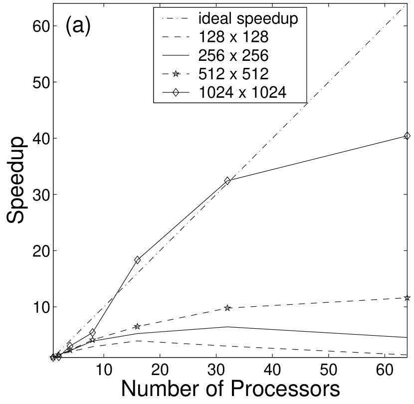
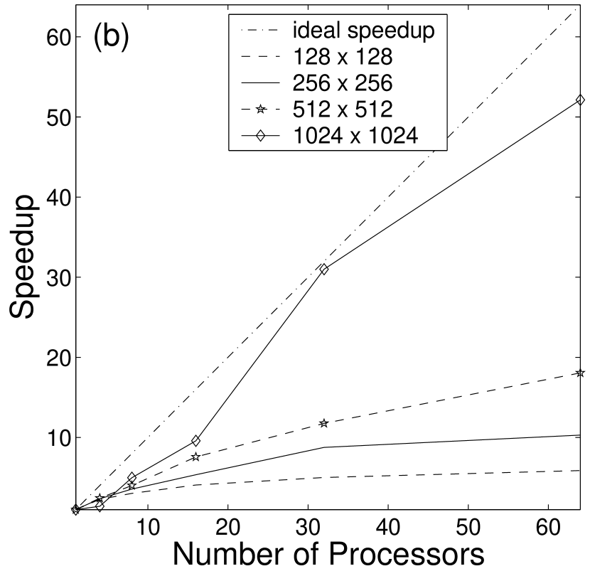
Figure 2: The speedup of 2D Navier-Stokes code with “2-n” scheme (a) and “4-n” scheme (b).

Figs. 2(a) shows the speedup plot for the 2-n scheme. For the resolution of $128^{2}$, the peak speed appears at 16 CPUs run (compared with 8 CPUs run for the 1-n scheme). For the resolution of $256^{2}$, the peak speed appears at 32 CPUs run (compared with 16 CPUs run for 1-n scheme). For $512^{2}$ and $1024^{2}$ in the 2-n scheme, and all the resolutions in the 4-n scheme (Fig. 2(b)), 64 CPUs run is the fastest.

Because two extra FFTs are introduced and $T_{sendrec}$ is slightly larger in 2-n and 4-n schemes, some runs in Figs. 2 are slower than the corresponding 1-n ones for certain resolution and $p$. For example, there is no super-linear speedup observed for the $1024^{2}$ curve in Fig. 2(b), although the 4-n scheme is twice as fast as the 1-n scheme when 64 processors are used.

In practice, the fastest scheme for fixed $p$ and $M^{2}$ is always what we want to use to do long time simulation. Fig.3 is a combined figure which consists of the best performance point in Figs. 1 and 2. Table 2 indicates the corresponding schemes adopted to draw this “best speedup” plot.

It should be emphasized that most points in the $1024^{2}$ curve show super-linear speedup. The points when $p\leq 16$ come from the 1-n scheme, while the 2-n and 4-n schemes are faster for $p\geq 32$.

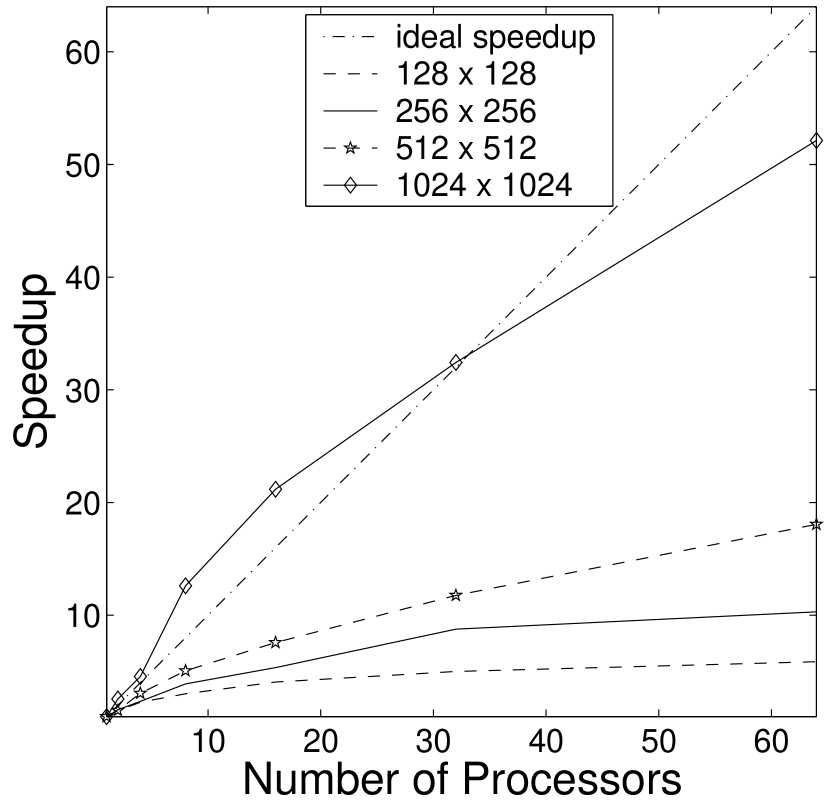
Figure 3: The speedup of 2D Navier-Stokes code with “ideal” scheme. The values used here are the top speedup among 1-n, 2-n, and 4-n scheme for same resolutions and same numbers of processors.

Table 2: The corresponding schemes for the values in Fig. 3.

	$128^{2}$	$256^{2}$	$512^{2}$	$1024^{2}$
1 CPU	1-n	1-n	1-n	1-n
2 CPUs	2-n	1-n	1-n	1-n
4 CPUs	4-n	4-n	1-n	1-n
8 CPUs	4-n	2-n	1-n	1-n
16 CPUs	4-n	4-n	4-n	1-n
32 CPUs	4-n	4-n	4-n	2-n
64 CPUs	4-n	4-n	4-n	4-n

For lower resolutions, the 1-n scheme works the best for small $p$, and the 2-n or 4-n scheme dominates the points on the corresponding curve in Fig.3 gradually for larger $p$. On the first column of Table 2, which corresponds to the resolution of $128^{2}$, the 4-n scheme dominates for $p\geq 4$.

The situations of $p=2$ in the 2-n scheme and $p=4$ in the 4-n scheme correspond to the PTD scheme. Although the benchmark results are slightly different from  [1] due to different computers used, the conclusion is the same: PTD is an easily implemented and efficient parallel scheme for the 2D DNS for relatively small resolutions.

The easy implementary property of PTD is inherited by PTF schemes: once the PFFT code is ready, it is very easy to change it to PTF codes. Hence, PTF is an attractive strategy, especially in 2D simulations.

2.4 Numerical results for 2D decaying turbulence

In this subsection, we will use our PTF codes to investigate an interesting phenomenon in 2D decaying turbulence – the multi-valued $\omega$-$\psi$ structure.

It is well known that if there is a functional relation $\omega=f(\psi)$, then the nonlinear term in Eq. (3) gives:

$${\rm{\bf u}}\cdot\nabla\omega=\frac{\partial\psi}{\partial y}\frac{\partial\omega}{\partial x}-\frac{\partial\psi}{\partial x}\frac{\partial\omega}{\partial y}=\frac{\partial f(\psi)}{\partial x}\frac{\partial\psi}{\partial y}-\frac{\partial f(\psi)}{\partial y}\frac{\partial\psi}{\partial x}=(\frac{\partial f}{\partial\psi}\frac{\partial\psi}{\partial x})\frac{\partial\psi}{\partial y}-(\frac{\partial f}{\partial\psi}\frac{\partial\psi}{\partial y})\frac{\partial\psi}{\partial x}=0.$$ (20)

Thus Eq. (3) becomes

$$\frac{\partial\omega}{\partial t}=\nu\Delta\omega.$$ (21)

For very high Reynolds number or $\nu\to 0$, Eq. (21) turns to a stationary equation

$$\frac{\partial\omega}{\partial t}=0.$$ (22)

It is common to treat $\omega=f(\psi)$ as an indication of the final state of 2D turbulence, but the simulation shown in Figs. 18-19 of Ref  [18] gives a counter example: the double-valued $\omega$-$\psi$ structure (see  [19] for a detailed discussion about this kind of structure). We will seek some other simulations to validate the generality of multi-valued structures, and there are mainly two choices to do this:

• Make changes in the initial conditions;

• Test different values of $\nu$ for certain kind of initial condition.

The parallel code we used before (PTD scheme  [1]) has a very limited speedup because the maximum number of CPUs used is limited to six. Most simulations were carried out by changing the initial condition for relatively small $\nu$ with the resolution of $512^{2}$  [19], which normally last from several days to a few weeks. For $1024^{2}$ runs, the calculations for one time step are four times as large as those for $512^{2}$, and the time step has to be smaller due to the CFL condition. A typical 2D decaying turbulence lasts from two months to half year if we only use PTD schemes. With the PTF codes, it is now possible to carry out $1024^{2}$ simulations to find the new double-valued $\omega$-$\psi$ structure.

We carried out two simulations starting from four equal sized vortices patches, which are asymmetrically placed in a double periodic box (Fig. 4). The first run adopted relatively low Reynolds number ($1/\nu=4000$) with the resolution of $512^{2}$. The time step is 0.0005. We used 32 CPUs in total (this is the maximum nodes available for long time simulations in LSEC). According to Table 2, the 4-n scheme is the fastest approach under this situation. The simulation lasted for 17 hours, and reached the quasi-steady state at $t\approx 200$ (Fig. 5(a)). Fig. 5(b) shows a simple function relation of $\omega$-$\psi$. The same run lasts for 29 hours if we use the PFFT scheme (32 CPUs), and 82 hours for the PTD scheme (4 CPUs).

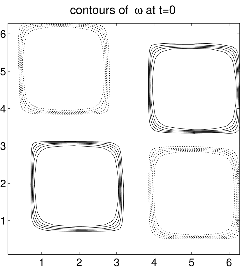
Figure 4: Contour plot of the initial condition in a simulation of Navier-Stoke equation which is initialized by two positive and two negative flat vortices (these four vortices are placed asymmetrically in the flow field). Dashed contours represent positive vorticity and drawn contours represent negative vorticity.

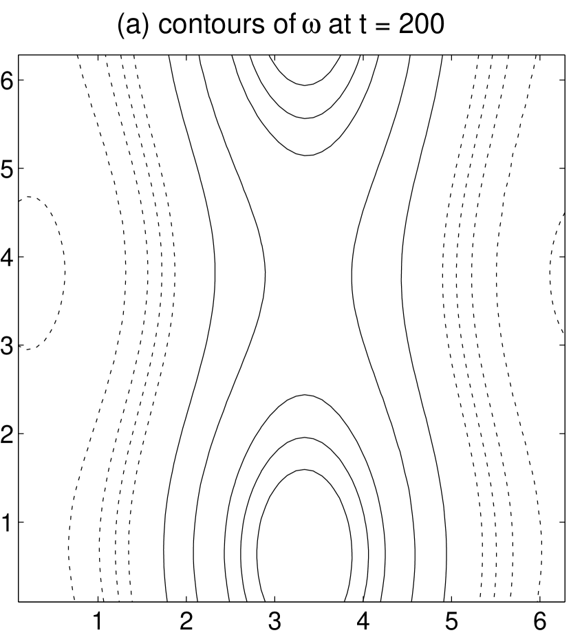
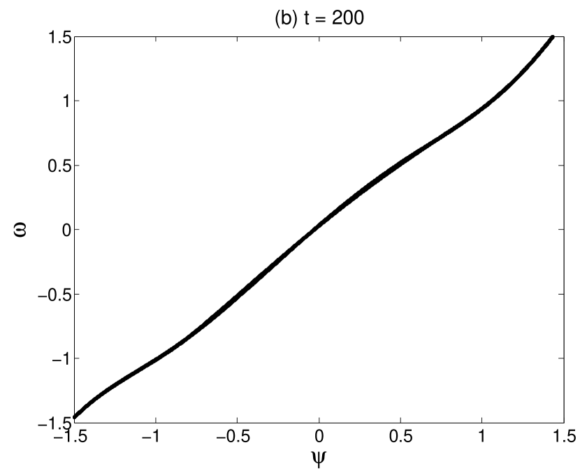
Figure 5: (a) is the vorticity contour plot at $t=200$ evolving from the initial condition shown in Fig. 4 (Re=4000). The resolution adopted is $512^{2}$. (b) is the $\omega$-$\psi$ scatter plot at the same time, which shows a simple functional relation.

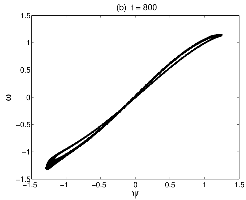
Figure 6: (a) is the vorticity contour plot at $t=800$ evolving from the initial condition shown in Fig. 4 (Re=40000). The resolution adopted is $1024^{2}$. (b) is the $\omega$-$\psi$ scatter plot at the same time, which shows a double-valued structure.

The second run adopted a large Reynolds number ($1/\nu=40000$) with the resolution of $1024^{2}$. We used the 2-n scheme code on 32 processors, and the quasi-steady state was reached at $t\approx 800$ after 16 days’ calculation. In the late state of this simulation, the orientation of the flow pattern is totally different from that obtained with the $512^{2}$ run (Fig. 6(a)). Moreover, the double-valued $\omega$-$\psi$ structure is recovered (Fig. 6(b)), which fits the definition of the final state of the 2D turbulence given in  [19]. Hence, it seems that further computations do not lead to any new phenomenon. The same run lasts for 20 days if we use the PFFT scheme (32 nodes), and about one year for the PTD scheme (4 nodes).

It is interesting to see the appearance of multi-valued $\omega$-$\psi$ structures in high Reynolds number (40000), while relatively low Reynolds number (4000) leads to traditional functional relation. Although the physical mechanism of the multi-valued structure is still unclear, our simulations reveal some limitations of the statistical mechanics [19], and it is worthwhile to carry on further investigations in this direction. Of course, the PTF scheme may play an important role in these large scale computations because of its high parallel efficiency.

With maximum 32 processors available for long time simulation, the peak speed of PFT is only about 70% faster than that of PFFT for the resolution of $512^{2}$, and 24% for $1024^{2}$. However, for runs like what are shown in Figs. 6, 24% shortage still means 4 days’ calculation on 32 nodes, which is definitely nontrivial.

3 Application of PTF scheme to 2D inviscid Boussinesq equations

It is very interesting to understand whether a finite time blow-up of the vorticity and temperature gradient can happen from a smooth initial condition in 2D inviscid Boussinesq convection. This has been studied recently by several groups ending with different conclusions: Pumir and Siggia used the TVD scheme with the adaptive meshes (the maximum grid size is $256^{2}$), which observed the blow-up process  [20]; E and Shu did not obtain the blow-up phenomena using the ENO scheme on a $512^{2}$ grid and spectral methods on a $1500^{2}$ grid  [21]; and Ceniceros and Hou also obtained blow-up free solutions using the adaptive mesh computation with a $512^{2}$ grid [22]. It is worth mentioning that the maximum mesh compression ratio in [22] is 8.83, which gave an effective resolution of $4600^{2}$ on uniform mesh. Although those groups yielded different conclusions, they all tried to use the highest possible resolutions to investigate the problem. Hence, parallel computing is a natural choice.

The 2D inviscid Boussinesq convection equations can be written in $\omega$-$\psi$ formulation:

$$\rho_{t}+{\rm{\bf u}}\cdot\nabla\rho=0,$$ (23)

$$\omega_{t}+{\rm{\bf u}}\cdot\nabla\omega=-\rho_{x},$$ (24)

$$\Delta\psi=-\omega.$$ (25)

Again, ABCN scheme is adopted to carry out the time integration. Below we will discuss how to implement our parallel strategy for Eqs. (23) - (25). Numerical results on the finite time blow-up will be reported.

3.1 The application of the new strategy to Boussinesq equations

As shown in Table 3, there are 20 FFTs involved when the Fourier-Galerkin spectral methods are used to solve Eqs. (23)-(25). These FFTs can be divided into four independent groups, which are indicated by the different columns in Table 3. There is no communication within the different columns until all FFTs are finished. In each column, the 1^st and the 2^nd FFT need to be evaluated before the 4^th one, while the 5^th FFT should be calculated after the 1^st and 3^rd one are finished.

Table 3: Twenty FFTs need to be calculated in each time step of Boussinesq spectral solver.

	A	B	C	D
1	$\hat{\mbox{u}}\to\mbox{u}$	$\hat{\mbox{U}}\to\mbox{U}$	$\hat{\mbox{v}}\to\mbox{v}$	$\hat{\mbox{V}}\to\mbox{V}$
2	$\hat{\omega}_{x}\to\omega_{x}$	$\hat{\Omega}_{x}\to\Omega_{x}$	$\hat{\omega}_{y}\to\omega_{y}$	$\hat{\Omega}_{y}\to\Omega_{y}$
3	$\hat{\rho}_{x}\to\rho_{x}$	$\hat{P}_{x}\to P_{x}$	$\hat{\rho}_{y}\to\rho_{y}$	$\hat{P}_{y}\to P_{y}$
4	$\mbox{u}\omega_{x}\to\widehat{\left({\mbox{u}\omega_{x}}\right)}$	$\mbox{U}\Omega_{x}\to\widehat{\left({\mbox{U}\Omega_{x}}\right)}$	$\mbox{v}\omega_{y}\to\widehat{\left({\mbox{v}\omega_{y}}\right)}$	$\mbox{V}\Omega_{y}\to\widehat{\left({\mbox{V}\Omega_{y}}\right)}$
5	$\mbox{u}\rho_{x}\to\widehat{\left({\mbox{u}\rho_{x}}\right)}$	$\mbox{UP}_{x}\to\widehat{\left({\mbox{UP}_{x}}\right)}$	$\mbox{v}\rho_{y}\to\widehat{\left({\mbox{v}\rho_{y}}\right)}$	$\mbox{VP}_{y}\to\widehat{\left({\mbox{VP}_{y}}\right)}$

Table 4: In 8-N scheme, the total twenty four FFTs in each time step of Boussinesq spectral solver are divided into eight groups (A-H). There are four FFTs introduced in addition to the twenty FFTs in Table 3.

	A	B	C	D
1	$\hat{\mbox{u}}\to\mbox{u}$	$\hat{\mbox{U}}\to\mbox{U}$	$\hat{\mbox{v}}\to\mbox{v}$	$\hat{\mbox{V}}\to\mbox{V}$
2	$\hat{\omega}_{x}\to\omega_{x}$	$\hat{\Omega}_{x}\to\Omega_{x}$	$\hat{\omega}_{y}\to\omega_{y}$	$\hat{\Omega}_{y}\to\Omega_{y}$
3	$\mbox{u}\omega_{x}\to\widehat{\left({\mbox{u}\omega_{x}}\right)}$	$\mbox{U}\Omega_{x}\to\widehat{\left({\mbox{U}\Omega_{x}}\right)}$	$\mbox{v}\omega_{y}\to\widehat{\left({\mbox{v}\omega_{y}}\right)}$	$\mbox{V}\Omega_{y}\to\widehat{\left({\mbox{V}\Omega_{y}}\right)}$
	E	F	G	H
1	$\hat{\mbox{u}}\to\mbox{u}$	$\hat{\mbox{U}}\to\mbox{U}$	$\hat{\mbox{v}}\to\mbox{v}$	$\hat{\mbox{V}}\to\mbox{V}$
2	$\hat{\rho}_{x}\to\rho_{x}$	$\hat{P}_{x}\to P_{x}$	$\hat{\rho}_{y}\to\rho_{y}$	$\hat{P}_{y}\to P_{y}$
3	$\mbox{u}\rho_{x}\to\widehat{\left({\mbox{u}\rho_{x}}\right)}$	$\mbox{UP}_{x}\to\widehat{\left({\mbox{UP}_{x}}\right)}$	$\mbox{v}\rho_{y}\to\widehat{\left({\mbox{v}\rho_{y}}\right)}$	$\mbox{VP}_{y}\to\widehat{\left({\mbox{VP}_{y}}\right)}$

When the PTF scheme is used to parallelize the code, there are five options to divide the groups without too much extra data communication:

1. 1 - N scheme – one group; each FFT is computed by all the CPUs involved, i.e. PFFT scheme. (Here we use “N” instead of “n” to avoid conflicts with the parallel schemes for the NS equations).

2. 2 - N scheme – two groups; column A & B in one group, and column C & D in the other group.

3. 4 - N scheme – four groups, which belongs to different columns in Table 3, respectively.

4. 8 - N scheme – eight groups, see column A-H of Table 4. Note that there are four extra FFTs introduced to save the communication time:. The first row FFTs in Table 3 are calculated twice in the first row of Table 4.

5. 12 - N scheme – twelve groups; the first three rows FFTs in Table 3 are calculated simultaneously in twelve groups, the results from the four groups calculating the first row FFTs are transferred to the eight groups computing the 2^nd and 3^rd row respectively, and the rest eight FFTs in the 4^th and 5^th rows are performed in those eight groups. (Like the 6-n scheme in the NS solver, the 12-N scheme will not be discussed here because the number of processors involved is not of the power of 2.)

Similar to Section 2, we will analyze the total computation time for different schemes in the following:

• 1-N scheme, 20 FFTs are involved:

  $$\textstyle\begin{array}[]{l}T_{sum}=20\times(p-1)\times 2\times\frac{\textstyle M^{2}}{\textstyle p^{2}}\times t_{sendrec}+20\times(p-1)\times 2\times t_{delay}\\ \quad\,\,\,\,+\frac{\textstyle 20}{\textstyle p}\times\left({M^{2}\log_{2}\left({M^{2}}\right)\;t_{c}}\right)\\ \quad\,\,\,\,=(40p-40)\times\frac{\textstyle M^{2}}{\textstyle p^{2}}\times t_{sendrec}+(40p-40)\times t_{delay}+\frac{\textstyle 20}{\textstyle p}\times\left({M^{2}\log_{2}\left({M^{2}}\right)\;t_{c}}\right).\\ \end{array}$$ (26)

• 2-N scheme, 10 FFTs in each groups, and two blocks (there are two equations in the system - Eqs. (23) and (24)) of $\frac{\textstyle M^{2}}{\textstyle p/2}$ size data will be transferred between the master group and the slave group in the beginning and end parts of the time loop:

  $$\begin{array}[]{l}T_{sum}=\left[{10\times(\frac{\textstyle p}{\textstyle 2}-1)\times 2\times\frac{\textstyle M^{2}}{\textstyle\left({p/2}\right)^{2}}+2\times 2\times\frac{\textstyle M^{2}}{\textstyle p/2}}\right]\times t_{sendrec}\\ \quad\quad\quad+\left({10\times(\frac{\textstyle p}{\textstyle 2}-1)\times 2+2\times 2}\right)\times t_{delay}+\frac{\textstyle 10}{\textstyle p/2}\times\left({M^{2}\log_{2}\left({M^{2}}\right)\;t_{c}}\right)\\ \;\quad=(48p-80)\times\frac{\textstyle M^{2}}{\textstyle p^{2}}\times t_{sendrec}+(10p-16)\times t_{delay}+\frac{\textstyle 20}{\textstyle p}\times\left({M^{2}\log_{2}\left({M^{2}}\right)\;t_{c}}\right).\\ \end{array}$$ (27)

• 4-N scheme, 5 FFTs in each groups, and two blocks of $\frac{\textstyle M^{2}}{\textstyle p/4}$ size data will be transferred between the master group and the slave groups in the beginning and end parts of the time loop:

  $$\begin{array}[]{l}T_{sum}=\left[{5\times(\frac{\textstyle p}{\textstyle 4}-1)\times 2\times\frac{\textstyle M^{2}}{\textstyle\left({p/4}\right)^{2}}+2\times 2\times\log_{2}^{4}\times\frac{\textstyle M^{2}}{\textstyle p/4}}\right]\times t_{sendrec}\\ \quad\quad\quad+\left({5\times(\frac{\textstyle p}{\textstyle 4}-1)\times 2+2\times 2\times\log_{2}^{4}}\right)\times t_{delay}+\frac{\textstyle 5}{\textstyle p/4}\times\left({M^{2}\log_{2}\left({M^{2}}\right)\;t_{c}}\right)\\ \quad\quad=(72p-160)\times\frac{\textstyle M^{2}}{\textstyle p^{2}}\times t_{sendrec}+(\frac{\textstyle 5}{\textstyle 2}p-2)\times t_{delay}+\frac{\textstyle 20}{\textstyle p}\times\left({M^{2}\log_{2}\left({M^{2}}\right)\;t_{c}}\right).\\ \end{array}$$ (28)

• 8-N scheme, 3 FFTs in each group, and two blocks of $\frac{\textstyle M^{2}}{\textstyle p/8}$ size data will be transferred between the master group and the slave groups in the beginning and end parts of the time loop:

  $$\begin{array}[]{l}T_{sum}=\left[{3\times(\frac{\textstyle p}{\textstyle 8}-1)\times 2\times\frac{\textstyle M^{2}}{\textstyle\left({p/8}\right)^{2}}+2\times 2\times\log_{2}^{8}\times\frac{\textstyle M^{2}}{\textstyle p/8}}\right]\times t_{sendrec}\\ \quad\quad\quad+\left({3\times(\frac{\textstyle p}{\textstyle 8}-1)\times 2+2\times 2\times\log_{2}^{8}}\right)\times t_{delay}+\frac{\textstyle 3}{\textstyle p/8}\times\left({M^{2}\log_{2}\left({M^{2}}\right)\;t_{c}}\right)\\ \quad\quad=(144p-384)\times\frac{\textstyle M^{2}}{\textstyle p^{2}}\times t_{sendrec}+(\frac{\textstyle 3}{\textstyle 4}p+6)\times t_{delay}+\frac{\textstyle 24}{\textstyle p}\times\left({M^{2}\log_{2}\left({M^{2}}\right)\;t_{c}}\right).\\ \end{array}$$ (29)

For all the PTF discussed above (Eq. (26)-(29)), it is clear that $T_{delay}$ will take larger portion of $T_{sum}$ when $p$ becomes larger in those schemes. For fixed $p$, $T_{delay}$ will take smaller portion of $T_{sum}$ when more groups are adopted in the PTF schemes (e.g. 4-N or 8-N scheme). Hence, the 4-N and 8-N schemes have some advantage over the 1-N and 2-N schemes when $p$ is large. Some further discussions for Eqs. (26) - (29) will be continued in the next subsection together with the speedup plots (Figs.7).

Like the 2D NS equations (Eqs. (4) and (5)), Eq. (24) and (25) can also be written in the conservative form:

$$\rho_{t}+\nabla\cdot\left({\rho{\rm{\bf u}}}\right)=0,$$ (30)

$$\left({\rho\omega}\right)_{t}+\nabla\cdot\left({\rho\omega{\rm{\bf u}}}\right)=-\frac{1}{2}\left({\rho^{2}}\right)_{x}.$$ (31)

When the Fourier-Galerkin spectral methods are used to solve the equations above, Eq. (31) presents some problem because the time evolution step is carried out in spectral space: to get the value of $\hat{\omega}$ in the next time step, $\widehat{\left({\rho\omega}\right)}$ has to be transferred back to physical space so the new value can be obtained by using the relation $\omega={\left({\rho\omega}\right)}\mathord{\left/{\vphantom{{\left({\rho\omega}\right)}\rho}}\right.\kern-1.2pt}\rho$. Furthermore, there is an extra nonlinear term $-\frac{1}{2}\left({\rho^{2}}\right)_{x}$ in Eq. (33) which requires one extra FFT. The total number of FFTs in conservative form is the same as non-conservative form. Hence, unlike what we did for 2D NS equations in section 2, the non-conservative equations are solved here.

3.2 Benchmarks and comparisons

In this subsection, we will show the speedup plots of the Boussinesq equations on SGI3800. Unlike what we did for the NS equations, we added a new resolution ($64^{2}$) to show the effectiveness of the new parallel scheme in the low resolution. The maximum processors used here is 32, which makes the resulting speedup plots (Figs. 7) more concise. It is also easier to use less than 32 processors in our 64-nodes machine; because we have to shut all other computing jobs down if we want to do the 64 CPUs run.

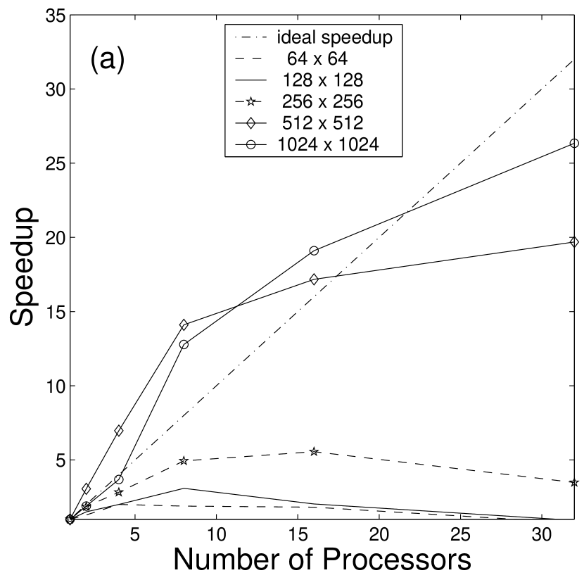
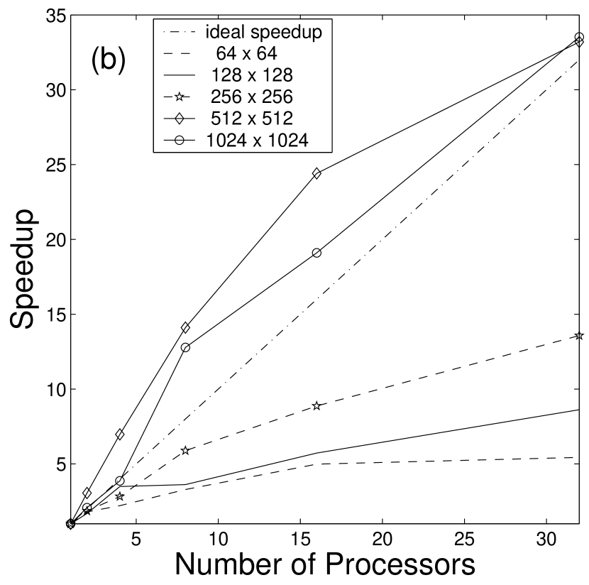
Figure 7: (a) The speedup of 2D Boussinesq code with PFFT scheme (or “1-N” scheme). (b) The speedup of 2D Boussinesq code with “ideal” scheme. The values used on (b) are the top speedup among 1-N, 2-N, 4-N, and 8-N scheme for same resolutions and same numbers of processors.

Fig. 7 (a) shows the speedup plot for PFFT (or. 1-N) scheme. The top speedup is obtained on 4 processors for the $64^{2}$ grid, while 8 and 16 processors reach the top speed for the resolutions of $128^{2}$ and $256^{2}$, respectively. The speedup curves of $512^{2}$ and $1024^{2}$ show reasonably good parallel efficiency of PFFT scheme. The $512^{2}$ runs show super linear speedup for 2, 4, 8, and 16 nodes, which is due to the cache effect. The $1024^{2}$ runs only have super linear speedup in the cases of 8 and 16 nodes. The speedups of 32-nodes run for these two high resolutions are lower than 32 because $T_{delay}$ begins to dominate the total computation time.

We did not show the speedup plots for resolutions higher than $1024^{2}$ because of the limit of the maximum local memory. However, since solving the equations with the highest possible resolution is the main task of our research, we will discuss the parallel efficiency on those high resolutions ($2048^{2}$ and $4096^{2}$) in other ways later in the next subsection.

Fig. 7(b) shows the “best speedup” plot of PTF schemes. All the resolutions have their top speed in the 32 CPUs case. Moreover, almost all the points on the curves show super linear speedup for higher resolutions ($512^{2}$ and $1024^{2}$).

The peak speeds shown in Fig. 7(b) are increased by a factor of 27% ($1024^{2}$ resolution) to 171% ($64^{2}$ resolution) compared to the PFFT scheme. The lower resolutions get a higher factor because the limitation of the total CPUs available. We can predict that the factor of $1024^{2}$ resolution will be larger than 27% if the maximum number of CPUs used is larger than 32.

Table 5: The corresponding schemes for the values in Fig. 7(b).

	$64^{2}$	$128^{2}$	$256^{2}$	$512^{2}$	$1024^{2}$
1 CPU	1-N	1-N	1-N	1-N	1-N
2 CPUs	2-N	2-N	1-N	1-N	2-N
4 CPUs	2-N	2-N	1-N	1-N	2-N
8 CPUs	8-N	2-N	2-N	1-N	1-N
16 CPUs	8-N	8-N	2-N	2-N	1-N
32 CPUs	8-N	8-N	8-N	4-N	2-N

Table 5 shows the corresponding schemes to the points on the Fig. 7(b). PFFT (or, 1-N) scheme never show the best performance for resolutions of $64^{2}$ and $128^{2}$ for $p\geq 2$ (For $p=1$, 1-N is the only choice, which is not necessary for comparison). For resolutions higher than $256^{2}$, the 1-N scheme reaches the peak speed more frequently, especially for runs with fewer processors.

As indicated in Table 5, the PTF schemes with more groups (e.g. 4-N or 8-N scheme) have better speedup for lower resolutions and larger number of CPUs, while the schemes divided into fewer groups (e.g. 1-N or 2-N scheme) work best for higher resolutions and relatively smaller number of CPUs.

In the real programming efforts, we found that it is more convenient to fix the size of each group (instead of fixing $p$) because the size of main calculating arrays can be determined beforehand. The code will get the number of groups (1, 2, 4, or 8) at the initial stage of real runs, and distribute the 20 FFTs into different groups. Thus, the programming effort concerning the PFT scheme is trivial if the PFFT code is already available.

Attention should be drawn to the performance of the 2-N scheme, which occupy eight of the total thirty places in Table 5. In the $1024^{2}$ runs, the 2-N scheme is faster than the 1-N scheme on 2 and 4 nodes’ simulations, which is counter to the conclusion we made in the above paragraph. Although most of the weird speedup behaviors in parallel computing can be attributed to cache effect, this one presents some difficulties because normally the more CPUs are used to calculate one FFT, the smaller $t_{c}$ will be (see the discussion in Section 2.2). To explain this, we need to calculate the exact values of $T_{comm}$ for the 1-N and 2-N schemes in our analytical models (Eqs. (26) and (27)).

For the 1-N scheme,

$$T_{comm}=\left\{{{\begin{array}[]{*{20}c}{10M^{2}\times t_{sendrec}+40\times t_{delay}\quad\quad\mbox{if}\;p=2\hfill}\\ {7.5M^{2}\times t_{sendrec}+120\times t_{delay}\quad\,\mbox{if}\;p=4.\hfill}\\ \end{array}}}\right.$$

For the 2-N scheme,

$$T_{comm}=\left\{{{\begin{array}[]{*{20}c}{4M^{2}\times t_{sendrev}+4\times t_{delay}\quad\quad\mbox{if}\;p=2\hfill}\\ {7M^{2}\times t_{sendrev}+24\times t_{delay}\quad\;\,\mbox{if}\;p=4.\hfill}\\ \end{array}}}\right.$$

It is clear that all parts of $T_{comm}$ in the 2-N scheme are smaller than the 1-N scheme in the case of $p\leq 4$, although $T_{sendrec}$ of the 2-N scheme is larger than that of the 1-N scheme for $p\geq 8$. Again, we assume that $t_{c}$ remains roughly the same for different schemes. The complete explanation has to take “cache effect” into consideration.

3.3 Numerical results for the Boussinesq convection

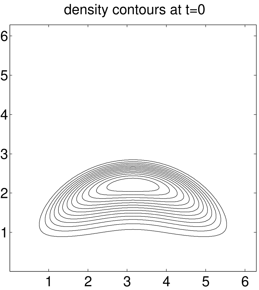
Figure 8: The contour plot of initial density, with the resolution of $1024^{2}$.

In this subsection, we will show some numerical simulations calculated by our parallel codes. For ease of comparison with former results, we adopted the same initial condition in Ref  [21]:

$$\omega(x,y,0)=0,$$ (32)

$$\rho(x,y,0)=50\rho_{1}(x,y)\rho_{2}(x,y)\left[{1-\rho_{1}(x,y)}\right],$$ (33)

where

$$\rho_{1}(x,y)=\left\{{{\begin{array}[]{*{20}c}{\exp\left({1-\frac{\textstyle\pi^{2}}{\textstyle\pi^{2}-x^{2}-(y-\pi)^{2}}}\right),\quad\mbox{if}\;x^{2}-(y-\pi)^{2}\leq\pi^{2},\hfill}\\ {0,\quad\quad\quad\mbox{otherwise,}\hfill}\\ \end{array}}}\right.$$

$$\rho_{2}(x,y)=\left\{{{\begin{array}[]{*{20}c}{\exp\left({1-\frac{\textstyle\left({1.95\pi}\right)^{2}}{\textstyle\left({1.95\pi}\right)^{2}-(x-2\pi)^{2}}}\right),\quad\mbox{if}\;\left|{x-2\pi}\right|\leq 1.95\pi,\hfill}\\ {0,\quad\quad\quad\mbox{otherwise.}\hfill}\\ \end{array}}}\right.$$

Fig. 8 shows the initial contour of $\rho$ on a grid of $1024^{2}$. The cap-like contour will develop into a rising bubble during the evolution, with the edge of the cap rolling up.

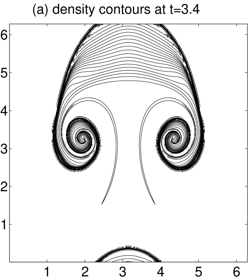
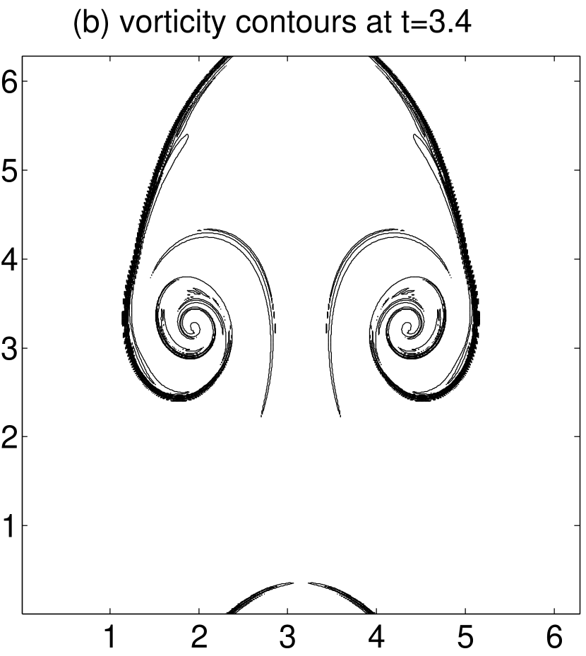
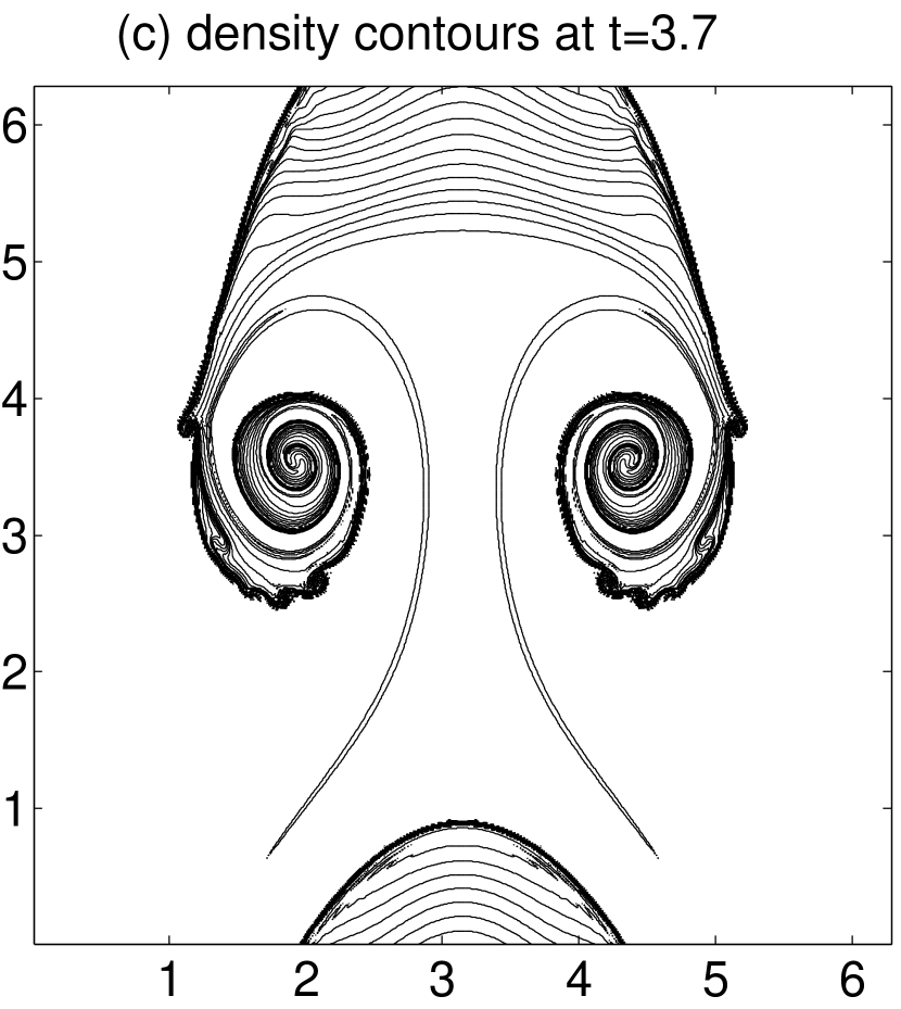
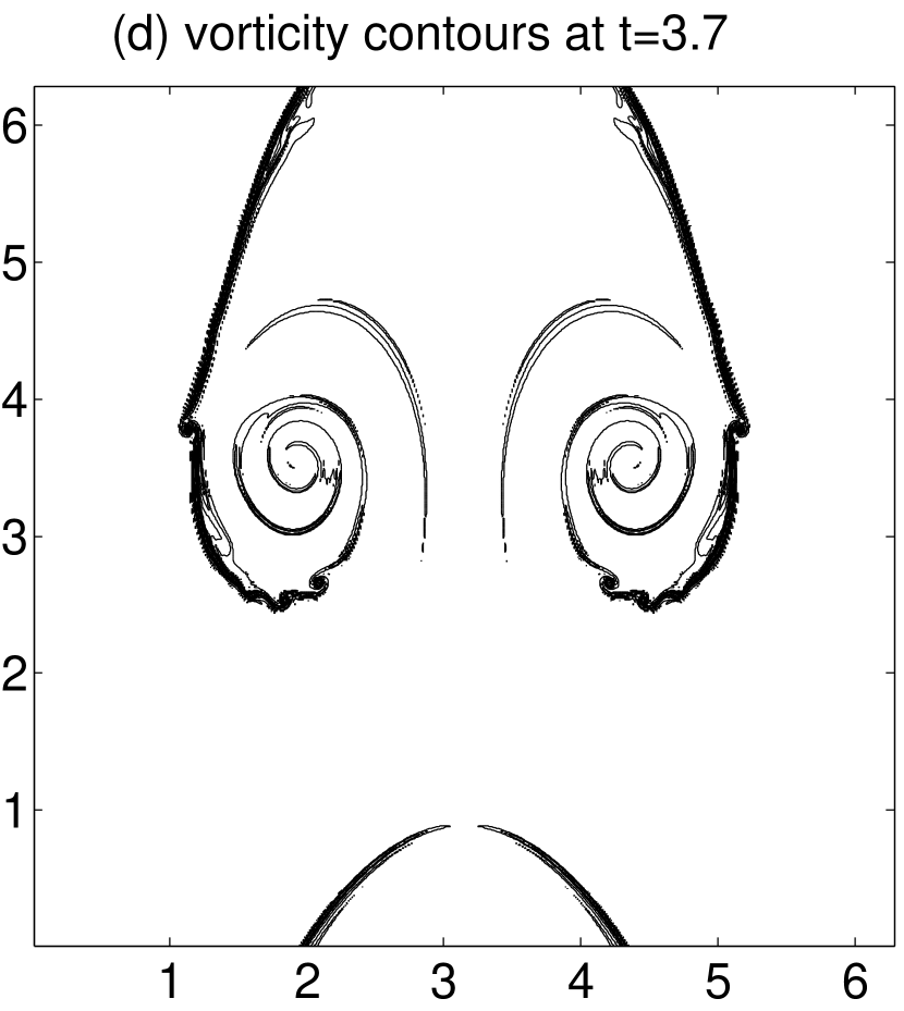
Figure 9: (a) and (b) show the contour plots of density and vorticity at t=3.4 with the resolution of $1024^{2}$, (c) and (d) show the contour plots at t=3.7.

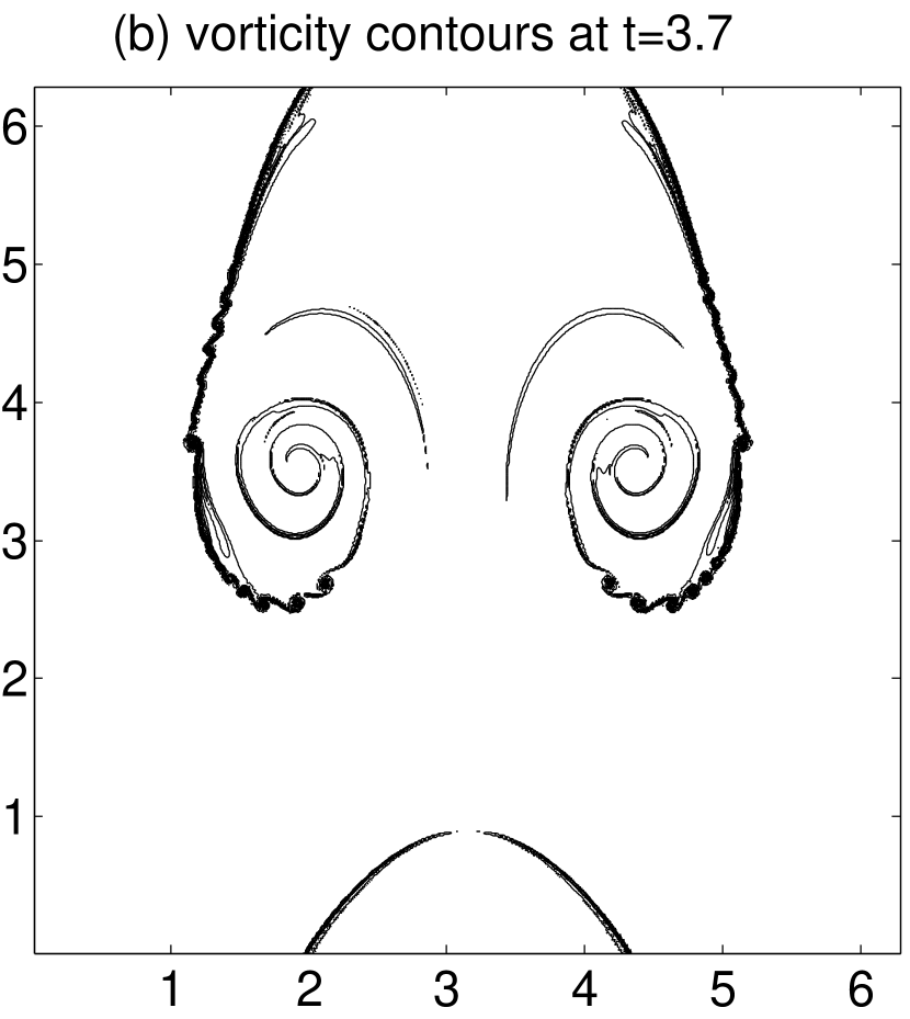
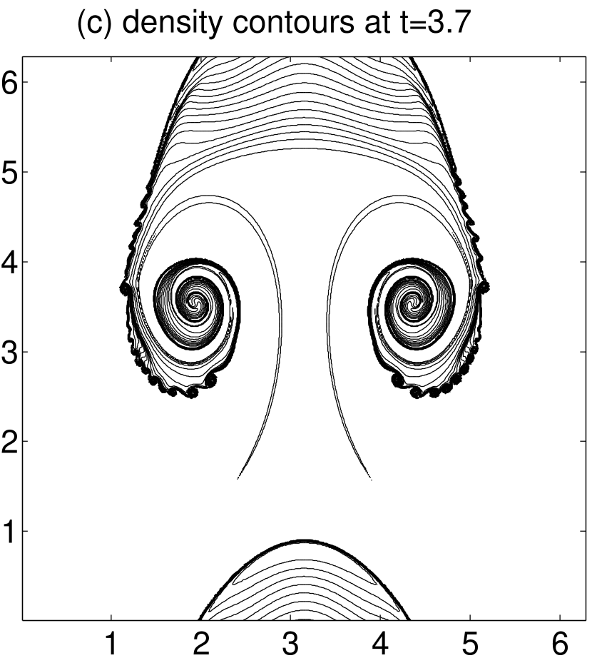
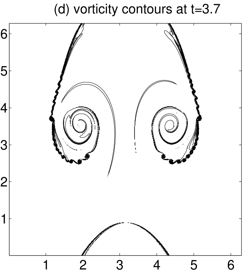
Figure 10: (a) and (b) are the contour plots of density and vorticity at t=3.7, with the resolution of $2048^{2}$. (c) and (d) are the contour plots with the resolution of $4096^{2}$ at t=3.7.

At $t\simeq 3.4$, the density and vorticity contour develop into the shape of “two eyes.” Figs. 9 (a) and (b) show the results with the resolution of $1024^{2}$. For spectral methods with different resolutions ($2048^{2}$ run of our simulation, and $1500^{2}$ run of  [21]) and ENO finite difference methods in  [21], some good agreements have been observed.

Arguments arise when the computations are carried on. At $t\simeq 3.7$, the smooth edge of the rolling eyes becomes unstable, see Figs. 9(c) and (d). Whether this phenomenon is physically real or not is still an open question. It was argued that this collapse is due to the numerical effect  [21, 22].

As discussed above, the most straightforward way to investigate this problem is to increase the resolution of simulations. Therefore, we also adopted grids of $2048^{2}$ and $4096^{2}$ in the simulations.

For the $1024^{2}$ run, the time step used is 0.0008 which is determined by the CFL condition. It took the parallel 2-N scheme twenty hours to reach $t=3.7$ with 32 processors. It takes 25 hours for PFFT schemes, and 28 days for the serial code.

For the $2048^{2}$ run, the time step used is 0.0004. The speed of the 1-N scheme and the 2-N scheme with 32 nodes are very close (a difference of 2%). We use the 1-N scheme because it is slightly faster. The code lasts for 13 days before it reaches $t=3.7$. For serial code, it may take one year provided the memory of the computer is large enough.

For the $4096^{2}$ run, the time step used is 0.0002. The 1-N scheme is the only choice because other schemes require larger computer memory: in principle, the memory size of the 2-N, 4-N, and 8-N schemes are 2, 4, and 8 times as large as that of the 1-N scheme. For this run, it is even a burdensome job for the parallel computation with 32 processors, which may last for four months in total. We actually use the interpolated data of the $2048^{2}$ run at $t=3.4$ as the initial condition. It is believed that the solution at $t=3.4$ is smooth. The code lasts for three weeks before it reaches $t=3.7$.

Figs. 10(a, b) show contour plots of the $2048^{2}$ run at $t=3.7$, on which the collapse is observed in the smooth edge; the same phenomenon is observed in the $4096^{2}$ run (Figs. 10(c, d)). It is noticed that more rolling vortices are observed on the edge of the “eyes” in Fig. 10(a) than that in Fig. 9(c), and even more vortices appear in Fig. 10(c). There are some trivial differences if we make a detailed comparison within these three runs, but Figs. 9(c, d) and Figs. 10 clearly show that the collapsing process is not a non-physical phenomenon from the numerical artifacts. If we started the $4096^{2}$ run from $t=0$ using Eq. (32) and (33) to get the initial data, the contour plots might be slightly different from what we obtained in Figs. 10(c, d). The main task here is to determine the possibility of the collapse phenomenon, the potential small difference in the flow pattern will not hurt the general conclusion. Some further details of the physical phenomenon will be discussed in another work. Here, we will try to focus our topic on the parallel solver.

Unlike the simulations in Section 2, most of computations (two of the three) in this section use the traditional PFFT scheme mainly due to the limitation of the maximum CPU number. If more processors are available so that the computer memory presents no problem to the PTF scheme, then the speed of PTF will also be faster than PFFT.

4 Conclusions and discussions

To sum up, the PTF scheme takes the advantages of the PTD and PFFT schemes, and can increase peak speed of codes significantly. The PTF scheme works best for low resolution run, or relatively large resolution with large number of CPUs. For very high resolutions, the PTF scheme is most likely slower than PFFT if not many processors are involved; PTF also needs more memory than that for PFFT, which presents some limitations on the scale of the highest resolution that one particular parallel computer can handle. These two disadvantages of PTF explain why similar schemes are not very popular in the 3D simulations where the array sizes may be even larger than that for the 2D simulations with high resolutions. It is advisable to treat PFFT as a special case of PTF, and the combined version of the parallel codes will always yield the best performance after a small amount of preparing work (e.g. making a table similar to Table 2 and Table 5 on the particular parallel machine to be used). In the meanwhile, the simple analytical mode of the parallel scheme, which divide $T_{sum}$ into three parts: $T_{sendrec}$, $T_{delay}$, and $T_{comp}$, is useful in explaining the performance of the parallel codes.

The parallel code of the NS equations helps us to find another example of double-valued $\omega$-$\psi$ structure; and the parallel Boussinesq code reveals the insight of an open question, which suggests that the collapse of the bubble cap may be a candidate for the finite time singularity formation. Both sets of investigation show that the parallel computing is useful in large scale numerical simulations.

We conclude our paper by some discussions on the future parallel computing. It is well-known that the speed of single processor increases much faster than the speed of memory access (five times faster in the last decade). Hence the latency of memory access in terms of processor clock cycle grows by a factor of five in the last ten years  [32]. For a fixed type of parallel scheme, the speedup curves (see Figs. 1-3 and 7) for high resolution (e.g. $1024^{2}$) in future machines may be similar to that of low resolutions in current computers ($64^{2}$ or $128^{2}$). In the case of PFFT scheme applied on a $1024^{2}$ resolution, it is possible that the speed of 64-nodes run is slower than that of the serial code in the future. On the other hand, the PTF scheme which uses much less $T_{delay}$ than that of the PFFT scheme has greater advantage over the PFFT scheme in parallel computing. In other words, the PTF strategy is also a scheme for the future.

Acknowledgments. We would like to thank Linbo Zhang, Zhongze Li, and Ying Bai for the support of using local parallel computers. ZY also thanks Prof. W.H. Matthaeus who supplied the original serial FORTRAN 77 Navier-Stokes pseudospectral codes. TT thanks the supports from International Research Team on Complex System, Chinese Academy of Sciences, and from Hong Kong Research Grant Council.

References

- [1] Z. Yin, H.J.H. Clercx, and D.C. Montgomery, An easily implemented task-based parallel scheme for the Fourier pseudospectral solver applied to 2D Navier-Stokes turbulence, Comput. Fluids, 33, 509 (2004).
- [2] S.A. Orszag, Accurate solution of the Orr-Sommerfeld stability equation, J.Fluid Mech., 50, 689, (1971)
- [3] G.S. Patterson and S.A. Orszag, Spectral calculations of isotropic turbulence: Efficient removal of aliasing interaction, Phys. Fluids, 14, 2538, (1971).
- [4] C. Canuto, M.Y. Hussaini, A. Quarteroni, and T.A. Zang, Spectral methods in fluid dynamics, Springer, New York, Berlin, 1987.
- [5] J. P. Boyd, Chebyshev and Fourier Spectral Methods, 2nd ed., Dover, Mineola/New York, 2001.
- [6] S. Chen, G.D. Doolen, R.H. Kraichnan, and Z. She, On statistical correlations between velocity increments and locally averaged dissipation in homogeneous turbulence, Phys. Fluids A, 5, 458 (1993).
- [7] Y. Kaneda, T. Ishihara, M. Yokokawa, K. Itakura, and A. Uno, Energy dissipation rate and energy spectrum in high resolution direct numerical simulations of turbulence in a periodic box, Phys. Fluids, 15, L21 (2003).
- [8] P. Moin and K. Mahesh, Direct numerical simulation: a tool in turbulence research, Annu. Rev. Fluid Mech., 30, 539 (1998).
- [9] R.B. Pelz, The parallel Fourier pseudospectral method, J. Comput. Phys., 92, 296, (1991).
- [10] E. Jackson, Z. She, and S.A. Orszag, A case study in parallel computing: I. Homogeneous turbulence on a hypercube, J. Sci. Comput., 6, 27, (1991).
- [11] P.F. Fischer and A.T. Patera, Parallel simulation of viscous incompressible flows, Annu. Rev. Fluid Mech., 26, 483 (1994)
- [12] M. Briscolini, A parallel implementation of a 3-D pseudospectral based code on the IBM 9076 scalable POWERparallel system, Parallel Comput., 21, 1849, (1995).
- [13] P. Dmitruk, L.P. Wang, W.H. Matthaeus, R. Zhang, and D. Seckel, Scalable parallel FFT for spectral simulations on a Beowulf cluster, Parallel Comput., 27, 1921, (2001).
- [14] M. Iovieno, C. Cavazzoni, and D. Tordella, A new technique for a parallel dealiased pseudospectral Navier-Stokes code, Comp. Phys. Commun., 141,365,(2001).
- [15] A.J. Basu, A parallel algorithm for spectral solution of the three-dimensional Navier-Stokes equations, Parallel Comput., 20, 1191, (1994).
- [16] W. Ling, J. Liu, J.N. Chung, and C.T. Crowe, Parallel algorithms for particles-turbulence two-way interaction direct numerical simulation, J. Parallel Distributed Comput., 62, 38, (2002).
- [17] E. Fournier, S. Gauthier, and F. Renaud, 2D pseudo-spectral parallel Navier-Stokes simulations of compressible Rayleigh-Taylor instability, Comput. Fluids, 31, 569 (2002).
- [18] Z. Yin, D.C. Montgomery, and H.J.H. Clercx, Alternative statistical-mechanical descriptions of decaying two-dimensional turbulence in terms of “patches” and “points,” Phys. Fluids, 15, 1937 (2003).
- [19] Z. Yin, On final states of two-dimensional decaying turbulence, Phys. Fluids, 16, 4623 (2003).
- [20] A. Pumir and E.D. Siggia, Development of singular solutions to the axisymmetric Euler equations, Phys. Fluids A, 4, 1472, (1992).
- [21] W. E and C. Shu, Small-scale structures in Boussinesq convection, Phys. Fluids, 6, 49, (1994).
- [22] H.D. Ceniceros and T.Y. Hou, An efficient dynamically adaptive mesh for potentially singular solutions, J. Comput. Phys., 172, 609,(2001).
- [23] D. Montgomery and G.R. Joyce, Statistical mechanics of negative temperature states, Phys. Fluids, 17, 1139, (1974).
- [24] C.Y. Chu, Comparison of two-dimensional FFT methods on the hypercube, in Proc. Third Confer. on Hypercube concurrent comput. Appl., Pasadena, California, United States, 1988, (ACM Press, New York, NY, USA, 1989), Vol. 2, pp. 1430.
- [25] P.N. Swarztrauber, Multiprocessor FFTs, Parallel Comput., 5, 197, (1987).
- [26] R.M. Chamberlain, Gray codes, Fast Fourier Transforms and hypercubes, Parallel Comput., 6, 225, (1988).
- [27] R.B. Pelz, Parallel compact FFTs for real sequences, SIAM J. Sci. Comput., 14, 914, (1993).
- [28] C. Mermer, D. Kim, and Y. Kim, Efficient 2D FFT implementation on mediaprocessors, Parallel Comput., 29, 691, (2003).
- [29] E. Chu and A. George, Inside the FFT black box, CRC Press, Boca Raton, London, New York, Washington, D.C., 2000.
- [30] D. Roose and R. Van Driessche, Parallel computers and parallel algorithms for CFD: an introduction, Special Course on Parallel Computing in CFD, AGARD R-807, NATO, 1995, pp. 1.1.
- [31] B.B. Fraguela, R. Doallo, J. Touriño, and E.L. Zapata, A compiler tool to predict memory hierarchy performance of scientific codes, Parallel Comput., 30, 225, (2004) (and references therein).
- [32] D.E. Culler, J.P. Singh, and A. Gupta, Parallel computer architecture, Morgan Kaufmann Publishers, Inc., San Francisco, 1999.