A new set of Monte Carlo moves for lattice random-walk models of biased diffusion

Abstract

We recently demonstrated that standard fixed-time lattice random-walk models cannot be modified to properly represent biased diffusion processes in more than two dimensions. The origin of this fundamental limitation appears to be the fact that traditional Monte Carlo moves do not allow for simultaneous jumps along each spatial direction. We thus propose a new algorithm to transform biased diffusion problems into lattice random walks such that we recover the proper dynamics for any number of spatial dimensions and for arbitrary values of the external field. Using a hypercubic lattice, we redefine the basic Monte Carlo moves, including the transition probabilities and the corresponding time durations, in order to allow for simultaneous jumps along all Cartesian axes. We show that our new algorithm can be used both with computer simulations and with exact numerical methods to obtain the mean velocity and the diffusion coefficient of point-like particles in any dimensions and in the presence of obstacles.

, ,

1 Introduction

Lattice Monte Carlo (LMC) computer simulations are often used to study diffusion problems when it is not possible to solve the diffusion equation. If the lattice mesh size is small enough, LMC simulations provide results that are in principle arbitrarily close to the numerical solution of the diffusion equation. In LMC simulations, a particle is essentially making an unbiased random-walk on connected lattice sites, and those moves that collide with obstacles are rejected [1, 2, 3, 4]. The allowed Monte Carlo moves are usually displacements by one lattice site along one of the $d$ spatial directions.

In the presence of an external field, one must bias the possible lattice jumps in order to also reproduce the net velocity of the particle. However, this is not as easy as it looks because one must also make sure that the diffusion coefficient is correctly modelled along each of the $d$ spatial directions. Using a Metropolis weighting factor [1] does not work because in the limit of large driving fields, all the jumps along the field axis are in the same direction and hence the the velocity saturates and the diffusion coefficient in this direction vanishes. This approach is thus limited to weak fields, at best. A better approach is to solve the local diffusion problem (i.e., inside each lattice cell) using a first-passage problem (FPP) [5, 6, 7, 8] approach, and to use the corresponding probabilities and mean jumping times for the coarser grained LMC moves. In this case, the mean jumping times are shorter along the field axis, but one can easily renormalize the jumping probabilities to use a single time step. In a recent paper [9], we demonstrated that although this method does give the correct drift velocity for arbitrary values of the driving field, it fails to give the correct diffusion coefficient. The problem is due to the often neglected fact that the variance of the jumping time affects the diffusion process in the presence of a net drift [10]. LMC models do not generally include these temporal fluctuations of the jumping time, at least not in an explicit way. In the same article [9], we showed how to modify a one-dimensional LMC algorithm with the addition of a stochastic jumping time $\tau\pm\Delta\tau$, where the appropriate value of the standard-deviation $\Delta\tau$ was again obtained from the resolution of the local FPP. For simulations in higher spatial dimensions $d>1$, it is possible to use our one-dimensional algorithm with the proper method to alternate between the dimensions as long as the Monte Carlo clock advances only when the particle moves along the field direction [9].

LMC simulations of diffusion processes actually use stochastic methods to resolve a discrete problem that can be written in terms of coupled linear equations. Several years ago, we proposed a way to compute the exact solution of the LMC simulations via matrix methods, thus bypassing the need for actual simulations. This alternative method is valid only in the limit of vanishingly weak driving fields, but it produces numerical results with arbitrarily high precision. The crucial requirement of the method is a set of LMC moves that have a common jumping time. Dorfman [11, 12] suggested a slightly different but still exact numerical method, and the two agree perfectly at zero-field. More recently [13], we extended our numerical method to cases with driving fields of arbitrary magnitudes; in order to do that, we used LMC moves that possess a single jumping time for all spatial directions, but this forced us to neglect the temporal fluctuations discussed above. As a consequence, our numerical method generates exact velocities but fails to provide reliable diffusion coefficients. Again, Dorfman’s alternate method also give the same velocities, but because the LMC moves do not include the proper temporal fluctuations, neither method can be used to compute the diffusion coefficient along the field axis. In summary, a fixed-time LMC algorithm can be used with exact numerical methods to compute the net velocity, but temporal fluctuations (and hence computer simulations) must be used to compute the diffusion coefficient.

We recently solved the problem of defining a LMC algorithm with both a fixed time step and the proper temporal fluctuations [9]. This required the addition of a probability to stay put on the current lattice site during a given time step (of course, this change also implies a renormalization of the jumping probabilities). This probability of non-motion has a direct effect on the real time elapsed between two displacements of the Brownian walker, and this effect can be adjusted in order to reproduce the exact temporal fluctuations of the local FPP. We showed that this new LMC algorithm can be used with Dorfman’s exact numerical method to compute the exact field-dependence of both the velocity and the diffusion coefficient of a particle on a lattice in the presence of obstacles. As far as we know, this is the first biased lattice random-walk model that gives the right diffusion coefficient for arbitrary values of the external field. Other models, such as the repton model [2], are restricted to weak fields. Several other articles (see, e.g. [14, 15, 16]) report simulations of diffusive processes, but all of them appear to be limited to small biases.

Unfortunately, our LMC algorithm [9] has a fatal flaw: for dimensions $d>2$, some of the jumping probabilities turn out to be negative. This failure suggests that there is a fundamental problem with this class of models, or more precisely with standard LMC moves (however, note that it is still possible to use computer simulations and fluctuating jumping times $\tau\pm\Delta\tau$, as explained above). In other words, it is impossible to get both the right velocity and the right diffusion coefficient in all spatial directions (if $d>2$) when the LMC jumps are made along a single axis at each step.

In this article, we examine an alternative to the standard LMC moves in order to derive a valid LMC algorithm with a common time step for spatial dimensions $d>2$. We suggest that a valid set of LMC moves should respect the fact that motion along the different spatial directions is actually simultaneous and not sequential. As we will show, this resolves the problem and allows us to design a powerful new LMC algorithm that can be used both with exact numerical methods and stochastic computer simulations.

2 The biased random-walk in one dimension

As mentioned above, Metropolis-like algorithms are not reliable if one wants to study diffusion via the dynamics of biased random-walkers on a lattice [9]. The discretization of such continuous diffusion processes should be done by first solving the FPP of a particle between two absorbing walls (the distance between these arbitrary walls is the step size $l$ of the lattice). Indeed, completion of a LMC jump is identical to the the first passage at a distance $l$ from the origin. In one dimension, this FPP has an exact algebraic solution, and the resulting transition probabilities (noted $\pm$ for parallel and antiparallel to the external force $F$) are [17]:

$$p_{\pm}(\epsilon)=\frac{1}{1+e^{\mp 2\epsilon}}\,,$$ (1)

where $\epsilon=Fl/2k_{B}T$ is the (scaled) external field intensity, $k_{B}$ is Boltzmann’s constant and $T$ is the temperature. The time duration of these FPP jumps is [17]:

$$\tau(\epsilon)=\frac{\tanh\epsilon}{\epsilon}\tau_{B}\,,$$ (2)

where $\tau_{B}$, the time duration $\tau(0)$ of a jump when no external field is applied, is called the Brownian time.

Although Eqs. 1 and 2 can be used to simulate one-dimensional drift problems (the net velocity is then correct), they erroneously generate a field-dependent diffusion coefficient for a free particle, which is wrong. This failure is due to the lack of temporal fluctuations in such a LMC algorithm (at each step, the particle would jump either forward ($p_{+}$) or backward ($p_{-}$), and all jumps would take the same time $\tau$). As mentioned above, it is possible to fix this problem [9] with a stochastic time step like $\tau\pm\Delta\tau$ where $\Delta\tau$ can also be calculated exactly within the framework of FPP’s [17]:

$$\Delta\tau(\epsilon)=\sqrt{\frac{\tanh\epsilon-\epsilon\,\mbox{sech}^{2}\epsilon}{\epsilon^{3}}}\times\tau_{B}\,.$$ (3)

However, the resulting algorithm can only be used in Monte Carlo computer simulations because exact resolution methods [13, 18] require a common time step for all jumps.

Alternatively, temporal fluctuations can be introduced using a probability $s^{\prime}$ to remain on the same lattice site during the duration of a fixed time step $\tau^{\prime}$ [9]. Not moving has for effect to create a dispersion of the time elapsed between two actual jumps. In order to obtain the right free-solution diffusion coefficient, we must have [9] :

$$s^{\prime}(\epsilon)=\frac{\coth\epsilon}{\epsilon}-\,\mbox{csch}^{2}\epsilon\,.$$ (4)

This modification also forces us to renormalize the other elements of the LMC algorithm:

$$p_{\pm}^{\prime}=(1-s^{\prime})p_{\pm}\,,$$ (5)

$$\tau^{\prime}=(1-s^{\prime})\tau\,.$$ (6)

Equations 4 to 6 define a LMC algorithm that can be used with Monte Carlo simulations (or exact numerical methods) to study one-dimensional drift and diffusion problems. One can easily verify [9] that it leads to the proper free-solution velocity ($v_{0}=\langle x\rangle/\tau^{\prime}=\epsilon l/\tau_{B}$) and diffusion coefficient ($D_{0}=\langle\Delta x^{2}\rangle/2\tau^{\prime}=l^{2}/2\tau_{B}$), while satisfying the Nernst-Einstein relation $D_{0}/v_{0}=l/\epsilon$. These equations will thus be the starting point of our new multidimensional LMC algorithm.

3 Extension to higher dimensions

In principle, we can build a simple model for $d>1$ dimensions using the elements of a one-dimensional biased random walk for the field axis and those of an unbiased random-walk for each of the $d-1$ transverse axes. Indeed, it is possible to fully decouple the motion along the different spatial directions if the field is along a Cartesian axis. Such an algorithm is divided into three steps:

1. First, we must select the jump axis, keeping in mind that the particle should share its walking time equally between the $d$ spatial directions. The probability to choose a given axis should thus be inversely proportional to the mean time duration of a jump in this direction (note that the time duration of a jump is shorter in the field direction).

2. Secondly, the direction ($\pm$) of the jump must be selected.

3. Finally, the time duration of the jump must be computed and the Monte Carlo clock must be advanced.

There are several ways to implement these steps. The easiest way is to use Eqs. 1 to 3; in this case, the LMC clock must advance by a stochastic increment $\tau\pm\Delta\tau$ each time a jump is made along the field axis (in order to obtain the proper temporal fluctuations, the clock does not advance otherwise). A slightly more complicated way would be to use Eqs. 4 to 6; again, the clock advances only when the jump is along the field axis, but this choice has the advantage of not needing a stochastic time increment. Although both of these implementations can easily be used with computer simulations, they would not function with exact numerical methods because of the way the clock is handled.

For exact numerical methods, an algorithm with a common time step and a common clock for all spatial directions is required. We showed that it is indeed possible to do this if we renormalize Eqs. 1 and 2 properly [13]; this approach works for any dimension $d>1$, but it can only be used to compute the exact velocity of the particle since it neglects the temporal fluctuations. In order to also include these fluctuations, one must start from Eqs. 4 to 6 instead. Unfortunately, this can be done only in two dimensions since the renormalization process gives negative probabilities when $d>2$ [9].

Clearly, in order to derive a multi-dimensional LMC algorithm with a fixed time-step, a common clock and the proper temporal fluctuations, we need a major change to the basic assumptions of the LMC methodology. In the next section, we propose to allow simultaneous jumps in all spatial directions. This is a natural choice since LMC methods do indeed assume that the motion of the particle is made of $d$ entirely decoupled random-walks. Current LMC methods assume this decoupling to be valid, but force the jumps to be sequential and not simultaneous.

4 The need for a new set of moves

In our multi-dimensional algorithm [9], the LMC moves were the standard unit jumps along one of the Cartesian axes, and a probability to stay put was used to generate temporal fluctuations. Since moving along a given axis actually contributes to temporal fluctuations along all the other axes [9], the method fails for $d>2$ because the transverse axes then provide an excess of temporal fluctuations. This strongly suggests that the traditional sequential LMC moves are the culprit. Sequential LMC moves are used solely for the sake of simplicity, but they are a poor representation of the fact that real particles move in all spatial directions at the same time. This weakness is insignificant for unbiased diffusion, but it becomes a roadblock in the presence of strong driving fields.

In order to resolve this problem, we thus suggest to employ a set of moves that respect the simultaneous nature of the dynamics along each of the $d$ axes. To generate a LMC algorithm for this new set of moves, we will use our exact solution of the one-dimensional problem for each of the $d$ directions.

5 New $d$-dimensional LMC moves: the free-solution case

Our new LMC moves will include one jump attempt along each of $d$ spatial directions. The list will thus consist of $d\,!\times 3^{d}$ different moves since we must allow for all possible permutations of the three fundamental jumps (of length $\pm l$ and $0$) used by the exact one-dimensional model that we will be using for each axis. Note that the external field must be parallel to one the Cartesian axes (we choose the $x$-axis here). The dynamics is governed by $p_{\pm}^{\prime}$, $s^{\prime}$ and $\tau^{\prime}$ in the $x$-direction (Eqs. 4 to 6), whereas we can in principle use $p_{\bot}=\frac{1}{2}$ and $\tau_{B}$ for the transverse directions because there is no need to model the temporal fluctuations when there is no net drift in the given direction [9].

The optimal time step for our new moves is $\tau^{\prime}(\epsilon)$, the duration of the fastest unit process. We thus have to rescale the transverse probability $p_{\bot}$ accordingly:

$$p_{\bot}^{\prime}=p_{\bot}\frac{\tau^{\prime}}{\tau_{B}}\,.$$ (7)

This generates an arbitrary probability to stay put in the transverse directions:

$$s_{\bot}^{\prime}=1-2p_{\bot}^{\prime}\,.$$ (8)

In the zero-field limit, this probability gives:

$$\left.s_{\bot}^{\prime}\right|_{\epsilon\rightarrow 0}=\frac{2}{3}=\left.s^{\prime}\right|_{\epsilon\rightarrow 0}\,.$$ (9)

Therefore, the probability to stay put is the same in all the directions in this limit, as it should. In the opposite limit $\epsilon\rightarrow\infty$, we have:

$$\left.s_{\bot}^{\prime}\right|_{\epsilon\rightarrow\infty}=1\,,$$ (10)

and the jumps in the transverse directions become extremely rare, as expected. Equations 4 to 8 are sufficient to build the table of multi-dimensional moves and their different probabilities since the $d$ directions are independent.

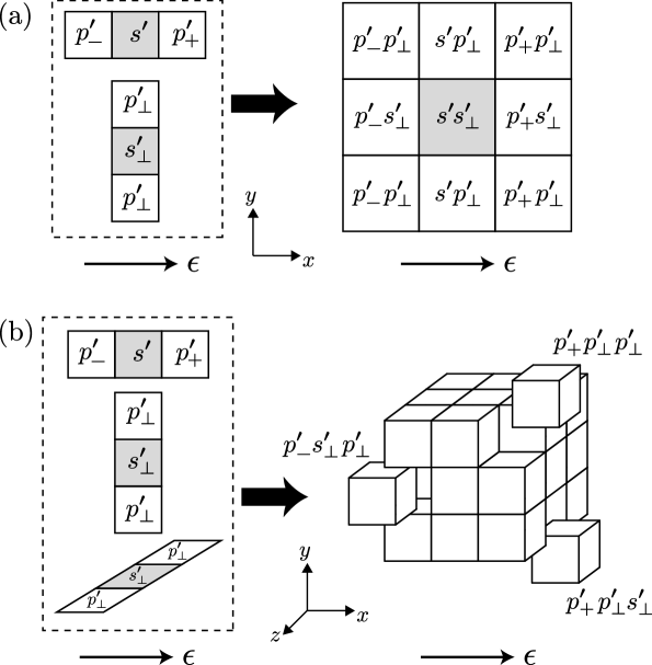
Figure 1: (a) Our new set of probabilities in two dimensions for an obstacle-free case (right) is the result of the combination of two simultaneous one-dimensional processes (left). The grey site represents the position of the random walker before the transition. (b) Same as in (a) for a three-dimensional system (for clarity, we present only three of the final transition probabilities).

Figure 1 illustrates the new LMC moves for the $2D$ and $3D$ cases in the absence of obstacles. The moves, all of duration $\tau^{\prime}$, combine $d$ simultaneous one-dimensional processes and include net displacements along lattice diagonals. The $d=2$ paths are further defined in Table 1a; such a description of the trajectories will be essential later to determine the dynamics in the presence of obstacles. It is straightforward to extend this approach to higher dimensions ($d>2$).

We can easily verify that this new set of LMC moves gives the right free-solution velocity and diffusion coefficients for all dimensions $d\geq 2$. If the field is pointing along the $x$-axis, the average displacement per time step is ${\langle X\rangle}^{\prime}=(p_{+}^{\prime}-p_{-}^{\prime})l$, while the average square displacement is ${\langle X^{2}\rangle}^{\prime}=(p_{+}^{\prime}+p_{-}^{\prime})l^{2}$. Using these results, we can compute the free-solution velocity $v_{0_{x}}$ and diffusion coefficient $D_{0_{x}}$:

$$v_{0_{x}}=\frac{{\langle X\rangle}^{\prime}}{\tau^{\prime}}=\frac{l\epsilon}{\tau_{B}}\,,$$ (11)

and

$$D_{0_{x}}=\frac{{\langle\Delta X^{2}\rangle}^{\prime}}{2\tau^{\prime}}=\frac{{\langle X^{2}\rangle}^{\prime}-{{\langle X\rangle}^{\prime}}^{2}}{2\tau^{\prime}}=\frac{l^{2}}{2\tau_{B}}\,.$$ (12)

One can also verify that $v_{0_{\bot}}=0$ and $D_{0_{\bot}}=l^{2}/2\tau_{B}$. These are precisely the results that we expect.

Therefore, the model introduced here does work for all values of the external field $\epsilon$ and all dimensions $d\geq 2$ in the absence of obstacles. The problems faced in Ref. [9] have been resolved by making the $d$ directions truly independent from each other and choosing $\tau^{\prime}$ as the fundamental time step of the new LMC moves.

6 New $d$-dimensional LMC moves: collisions with obstacles

Since this new model works fine in free-solution, the next step is to define how to deal with the presence of obstacles. The rule that we follow in those cases where a move leads to a collision with an obstacle is the same as before, i.e., such a jump is rejected and the particle remains on the same site. In our algorithm, though, this means that one (or more) of the $d$ sub-components of a $d$-dimensional move is rejected. Therefore, the list of transition probabilities must take into account all of the possible paths that the particle can follow given the local geometry. A two-dimensional example is illustrated in Table 1b. We see that the two different trajectories that previously lead to the upper right corner (site $c$) now lead to different final positions due to the rejection of one of the two unit jumps that are involved. The final transition probabilities for this particular case are listed in Table 1b. Of course, all local distributions of obstacles can be studied using the same systematic approach.

7 New $d$-dimensional LMC moves: the continuum limit

In order to test our new set of LMC moves for systems with obstacles, we will compare its predictions to those of our previous two-dimensional algorithm [9] since we know that both can properly reproduce the velocity and the diffusion coefficient of a particle in the case of an obstacle-free system. However, the different moves used by these two algorithms means that a true comparison can only be made in the limit of the continuum since the choice of moves always affects the result of a coarse-grained approach if there are obstacles.

The exact numerical method that we developed in collaboration with Dorfman [18] is not limited to the previous set of LMC moves. It can easily be modified to include other LMC moves, including diagonal moves. Combining Dorfman’s method [18, 11, 12] and our new LMC moves, we now have a way to compute the exact velocity and the exact diffusion coefficient of a particle in the presence of arbitrary driving field for any dimension $d\geq 2$.

We thus studied the system shown in Fig. 2b using both algorithms, and we repeated the calculation for different lattice parameters $\xi l$ (with $0<\xi\leq 1$) while the obstacle size ($l$) remained constant (the surface concentration of obstacles is thus kept constant at $C=1/9$). The limit of the continuum corresponds to $\xi\rightarrow 0$. We compared the velocities and diffusion coefficients along the field-axis obtained with both algorithms over a wide range of $\xi$. Note that the value of the external scaled field $\epsilon$, which is proportional to the lattice parameter ($\epsilon=Fl/2k_{B}T$), has to be rescaled by the factor $\xi$. Figure 2a presents the data for both algorithms for a nominal field intensity $\epsilon=1$. We clearly see that the two approaches converge perfectly in the $\xi\rightarrow 0$ limit. Interestingly, the new algorithm converges slightly faster towards the asymptotic continuum value. This is explained by the fact that the diagonal transitions reduce the number of successive collisions made by a random-walker when it is trapped behind an obstacle at high field.

8 Conclusion

Conventional three-dimensional LMC algorithms cannot be used to study both the mean velocity and the diffusion coefficient of a Brownian particle if the time step has to be constant (as required by exact numerical methods). This limitation is due to the fact that these algorithms only allow jumps to be made along one axis at each time step. Such unit jumps make it impossible to obtain the proper temporal fluctuations that are key to getting the right diffusion coefficient.

We propose that LMC moves should actually respect the fact that all of the $d$ spatial dimensions are fully independent. This means that each move should include a component along each of these dimensions. This complete dimensional decoupling allows us to conserve the proper temporal fluctuations and hence to reproduce the correct diffusion process even in the presence of an external field of arbitrary amplitude. This approach leads to a slightly more complicated analysis of particle-obstacle collisions, but this is still compatible with the exact numerical methods developed elsewhere [9].

The new LMC algorithm presented in this paper opens the door to numerous coarse-grained simulation and numerical studies that were not possible before because previous algorithms were restricted to low field intensities.

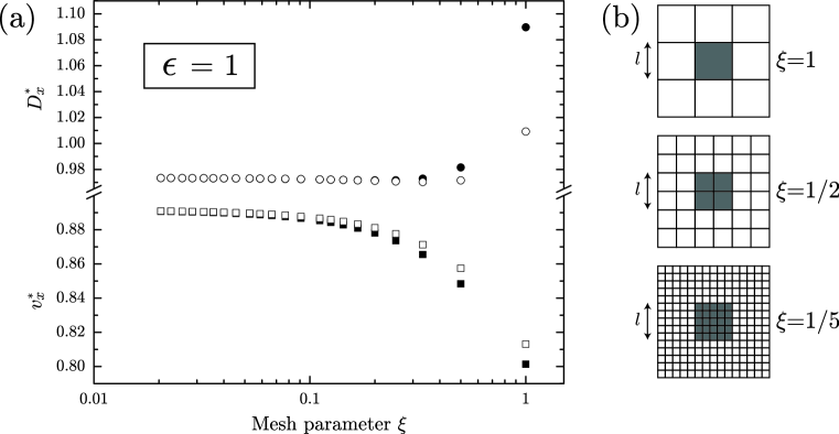
Figure 2: (a) Scaled velocity $v_{x}^{*}$ (squares) and diffusion coefficient $D_{x}^{*}$ (circles) vs the mesh size $\xi$ for $\epsilon=1$. These calculations were done using the algorithm presented in Ref. [18] (filled symbols) and the one proposed in this paper (empty symbols). (b) The obstacle is of size $l\times l$, the lattice is of size $3l\times 3l$ (with periodic boundary conditions), and the particle (not shown) is of size $\xi l\times\xi l$. The system is shown for three different values of the mesh size parameter $\xi$.

Table 1: Listing of all the possible trajectories and their transition probabilities in two dimensions for the free-solution case (a) and an example of obstacle obstruction (b).

(a) Free-solution case		(b) Obstacle case
$1^{st}$ jump $2^{nd}$ jump final position transition probability $p_{-}^{\prime}$ $p_{\bot}^{\prime}$ $p_{\bot}^{\prime}$ $p_{-}^{\prime}$ $a$ $p_{-}^{\prime}p_{\bot}^{\prime}$ $s^{\prime}$ $p_{\bot}^{\prime}$ $p_{\bot}^{\prime}$ $s^{\prime}$ $b$ $s^{\prime}p_{\bot}^{\prime}$ $p_{+}^{\prime}$ $p_{\bot}^{\prime}$ $p_{\bot}^{\prime}$ $p_{+}^{\prime}$ $c$ $p_{+}^{\prime}p_{\bot}^{\prime}$ $p_{-}^{\prime}$ $s_{\bot}^{\prime}$ $s_{\bot}^{\prime}$ $p_{-}^{\prime}$ $d$ $p_{-}^{\prime}s_{\bot}^{\prime}$ $s^{\prime}$ $s_{\bot}^{\prime}$ $s_{\bot}^{\prime}$ $s^{\prime}$ $e$ $s^{\prime}s_{\bot}^{\prime}$ $p_{+}^{\prime}$ $s_{\bot}^{\prime}$ $s_{\bot}^{\prime}$ $p_{+}^{\prime}$ $f$ $p_{+}^{\prime}s_{\bot}^{\prime}$ $p_{-}^{\prime}$ $p_{\bot}^{\prime}$ $p_{\bot}^{\prime}$ $p_{-}^{\prime}$ $g$ $p_{-}^{\prime}p_{\bot}^{\prime}$ $s^{\prime}$ $p_{\bot}^{\prime}$ $p_{\bot}^{\prime}$ $s^{\prime}$ $h$ $s^{\prime}p_{\bot}^{\prime}$ $p_{+}^{\prime}$ $p_{\bot}^{\prime}$ $p_{\bot}^{\prime}$ $p_{+}^{\prime}$ $i$ $p_{+}^{\prime}p_{\bot}^{\prime}$		$1^{st}$ jump $2^{nd}$ jump final position transition probability $p_{-}^{\prime}$ $p_{\bot}^{\prime}$ $p_{\bot}^{\prime}$ $p_{-}^{\prime}$ $a$ $p_{-}^{\prime}p_{\bot}^{\prime}$ $s^{\prime}$ $p_{\bot}^{\prime}$ $p_{\bot}^{\prime}$ $p_{\bot}^{\prime}$ $s^{\prime}$ $p_{+}^{\prime}$ $b$ $\displaystyle s^{\prime}p_{\bot}^{\prime}+\frac{p_{+}^{\prime}p_{\bot}^{\prime}}{2}$ $p_{-}^{\prime}$ $s_{\bot}^{\prime}$ $s_{\bot}^{\prime}$ $p_{-}^{\prime}$ $d$ $p_{-}^{\prime}s_{\bot}^{\prime}$ $s^{\prime}$ $s_{\bot}^{\prime}$ $s_{\bot}^{\prime}$ $s^{\prime}$ $e$ $s^{\prime}s_{\bot}^{\prime}$ $p_{+}^{\prime}$ $s_{\bot}^{\prime}$ $p_{+}^{\prime}$ $s_{\bot}^{\prime}$ $p_{+}^{\prime}$ $p_{\bot}^{\prime}$ $f$ $\displaystyle p_{+}^{\prime}s_{\bot}^{\prime}+\frac{p_{+}^{\prime}p_{\bot}^{\prime}}{2}$ $p_{-}^{\prime}$ $p_{\bot}^{\prime}$ $p_{\bot}^{\prime}$ $p_{-}^{\prime}$ $g$ $p_{-}^{\prime}p_{\bot}^{\prime}$ $s^{\prime}$ $p_{\bot}^{\prime}$ $p_{\bot}^{\prime}$ $s^{\prime}$ $h$ $s^{\prime}p_{\bot}^{\prime}$ $p_{+}^{\prime}$ $p_{\bot}^{\prime}$ $p_{\bot}^{\prime}$ $p_{+}^{\prime}$ $i$ $p_{+}^{\prime}p_{\bot}^{\prime}$

References

- [1] K. Binder and D. W. Heermann. Monte Carlo Simulation in Statistical Physics, 2nd Corrected Ed. Springer-Verlag, 1992.
- [2] M. E. J. Newman and G. T. Barkema. Monte Carlo Methods in Statistical Physics. Clarendin Press, 1999.
- [3] D. W. Heermann. Computer Simulation Methods in Theoretical Physics, 2nd Ed. Springer-Verlag, 1990.
- [4] K. Binder, editor. Monte Carlo and Dynamics Simulations in Polymer Science. Oxford University Press, 1995.
- [5] S. Redner. A Guide to First-Passage Processes. Cambridge University Press, 2001.
- [6] Z. Farkas and T. Fulop. One-dimensional drift-diffusion between two absorbing boundaries: application to granular segregation. J. Phys. A, 34:3191–3198, 2001.
- [7] N. G. van Kampen. Stochastic Processes in Physics and Chemistry, pages 347–355. North-Holland, 1992.
- [8] C. W. Gardiner. Handbook of Stochastic Methods for Physics, Chemistry, and the Natural Sciences. Springer-Verlag, 1983.
- [9] M. G. Gauthier and G. W. Slater. Building lattice random-walk models for real drift and diffusion problems. Phys. Rev. E, 70:015103(R), 2004.
- [10] J.-P. Bouchaud and A. Georges. Anomalous diffusion in disordered media - statistical mechanisms, models and physical applications. Phys. Rep., 195:127–293, 1990.
- [11] K. D. Dorfman. Exact computation of the mean velocity, molecular diffusivity, and dispersity of a particle moving on a periodic lattice. J. Chem. Phys., 118:8428–8436, 2003.
- [12] K. D. Dorfman, G. W. Slater, and M. G. Gauthier. Generalized taylor-aris dispersion analysis of spatially periodic lattice monte carlo models: Effect of discrete time. J. Chem. Phys., 119:6979–6980, 2003.
- [13] M. G. Gauthier and G. W. Slater. Exactly solvable Ogston model of gel electrophoresis: IX. Generalizing the lattice model to treat high field intensities. J. Chem. Phys., 117:6745–6756, 2002.
- [14] S. Havlin and D. Ben-Avraham. Diffusion in disordered media. Advances in Physics, 51:187–292, 2002.
- [15] M. Q. López-Salvans, J. Casademunt, G. Iori, and F. Sagués. Dynamics of finger arrays in a diffusion-limited growth model with a drift. Physica D, 164:127–151, 2002.
- [16] S. Bustingorry, E. R. Reyes, and M. O. Cáceres. Biased diffusion in anisotropic disordered systems. Phys. Rev. E, 62:7664–7669, 2000.
- [17] G. W. Slater. Theory of band broadening for DNA gel electrophoresis and sequencing. Electrophoresis, 14:1–7, 1993.
- [18] M. G. Gauthier, G. W. Slater, and K. D. Dorfman. Exact lattice calculations of dispersion coefficients in the presence of external fields and obstacles. Eur. Phys. J. E, 2004.