Abstract

Equilibrium eigenstates of an axisymmetric magnetically confined plasma with toroidal flow are investigated by means of exact solutions of the ideal magnetohydrodynamic equations. The study includes ”compressible” flows with constant temperature, $T(\psi)$, but varying density on magnetic surfaces and incompressible ones with constant density, $\varrho(\psi)$, but varying temperature thereon (the function $\psi(R,z)$ is the poloidal magnetic flux-function with $(R,z,\phi)$ cylindrical coordinates). These variations are necessary for the existence of tokamak steady states with flow. The ”compressible” and incompressible solutions are associated with the ansatz $\omega^{2}/T\propto M_{0}=\mbox{constant}$ and $d(\varrho\omega^{2})/d\psi=A\psi$, respectively, where $\omega(\psi)$ is the rotation frequency. In both cases eigenfunctions of the form $\psi_{\ell n}={\cal Z}_{\ell}(z){\cal R}_{n}(R)$ ($\ell,n=1,2,\ldots$) describe configurations with $\ell\times n$ magnetic axes. Owing to the flow, the respective eigenvalues can be considered in two alternative ways: either as flow eigenvalues, $M_{0}^{\ell}$ and $A^{\ell}$, which depend on a pressure parameter, $P_{0}$, or as pressure eigenvalues, $P_{0}^{\ell}$, which depend on the flow parameters $M_{0}$ or $A$. In the context of the latter consideration when the flow parameters are varied continuously there are transition points, $(M_{0})_{m}$ and $A_{m}$ ($m=1,2,\ldots$), at which an additional magnetic axis is formed. This flow-caused change in magnetic topology is possible solely in the presence of toroidicity because in the limit of infinite aspect ratio the axial flow does not appear in the equilibrium equation. Also, the lower the aspect ratio the smaller $(M_{0})_{m}$ and $A_{m}$. In addition, the effects of the flow and the aspect ratio on the Shafranov shift are evaluated.

I. Introduction

Over the last decades it has been established experimentally and theoretically that the flow affects the confinement properties of magnetically confined plasmas. In particular, the flow and especially the flow shear play a role in the formation of edge transport barriers (L-H transition) as well as of Internal Transport Barriers (ITBs), two enhanced confinement modes in tokamaks (e.g. see Ref. [1] and Refs. cited therein). Also, the majority of the advanced tokamak scenarios include flow. The ITBs usually are associated with reversed magnetic shear profiles. In addition, a possible magnetic topology of static (no-flow) equilibria with reversed current density in the core region proposed in Ref. [2] consists of multitoroidal configurations having non-nested magnetic surfaces.

Magnetohydrodynamic (MHD) equilibrium equations for axisymmetric magnetically confined plasmas with (a) isothermal magnetic surfaces and toroidal flow and (b) incompressible flow of arbitrary direction have been obtained in Ref. [3] and [4], respectively. Although purely toroidal axisymmetric flows are inherent incompressible because of symmetry, the former equilibria can be regarded as ”compressible” in the sense that, alike the latter ones, the density varies on magnetic surfaces. Respective exact solutions were constructed in Refs. [3, 5, 6] and [4, 7, 8] and the impact of flow on certain equilibrium characteristics was examined therein. In particular, in. Ref. [7] we extended the well known Solovév solution [9, 10] to unbounded incompressible plasmas and found that the flow and its shear can change the magnetic topology thus resulting in a variety of novel configurations of astrophysical and laboratory concern.

The aim of the present study is to examine the possible impact of the flow on the magnetic topology for equilibria relevant to plasmas of fusion devices. The study includes equilibria with both ”compressible” and incompressible toroidal flows. The main conclusion is that the flow in conjunction with toroidicity can change the magnetic structure by the formation of addition magnetic axes. The role of the toroidicity is important, i.e. this formation is not possible in the limit of infinite aspect ratio.

The outline of the report is as follows. A derivation of the ”compressible” and incompressible equilibrium equations in a unified manner is first reviewed and respective exact solutions are presented in Sec. II. In Sec. III equilibrium eigenstates of a magnetically confined plasma surrounded by a boundary of rectangular cross-section and arbitrary aspect ratio are constructed. On the basis of these eigenstates the impact of the flow on the magnetic topology is then studied in conjunction with the role of toroidicity. The effects of the flow and the aspect ratio on the Shafranov shift are examined in Sec. IV. Finally the conclusions are summarized in section V.

II. Equilibrium equations and solutions

The ideal axisymmetric MHD equilibrium equations for the cases of ”compressible” and incompressible toroidal flows are reviewed in this Section. In particular, a unified derivation is given without adopting from the beginning relevant energy equations or equations of states. They will be specified when necessary later. This rather detailed presentation aims at making the discussion in the subsequent sections tangible, particularly as concerns the role of toroidicity.

The starting equations written in standard notation and convenient units are the following:

$${\bf\nabla}\cdot(\varrho{\bf v})=0$$ (1)

$$\varrho({\bf v}\cdot{\bf\nabla}){\bf v}={\bf J}\times{\bf B}-{\bf\nabla}P$$ (2)

$${\bf\nabla}\times{\bf E}=0$$ (3)

$${\bf\nabla}\times{\bf B}={\bf J}$$ (4)

$${\bf\nabla}\cdot{\bf B}=0$$ (5)

$${\bf E}+{\bf v}\times{\bf B}=0$$ (6)

An energy equation or equation of state (7)

For axisymmetric magnetically confined plasmas with toroidal flow the divergence-free magnetic field and mass flow can be written in terms of the scalar functions $\psi(R,z)$, $I(R,z)$ and $K(R,z)$ as

$${\bf B}=I{\bf\nabla}\phi+{\bf\nabla}\phi\times{\bf\nabla}\psi$$ (8)

$$\varrho{\bf v}=K{\bf\nabla}\phi.$$ (9)

The toroidal current density is then put, by Amp$\acute{e}$re’s law, in the form

$${\bf J}={\bf\Delta}^{*}\psi{\bf\nabla}\phi-{\bf\nabla}\phi\times{\bf\nabla}I$$ (10)

Here ($R,\phi,z$) are cylindrical coordinates with $z$ corresponding to the axis of symmetry, $\psi$ labels the magnetic surfaces and ${\bf\Delta}^{*}$ is the elliptic operator defined as $R^{2}{\bf\nabla}\cdot({\bf\nabla}/R^{2})$.

By projecting the momentum equation (2) and Ohm’s law (6) along the toroidal direction, the magnetic field, and perpendicular to the magnetic surfaces some integrals are identified as flux functions, i.e. functions constant on magnetic surfaces, and Eqs. (1-6) are reduced to simpler ones. In particular, the $\nabla\phi$-component of (2) yields

$${\bf\nabla}\phi\cdot({\bf\nabla}\psi\times{\bf\nabla}I)=0$$ (11)

implying that $I=I(\psi)$. Also, expressing the electric field in terms of the electrostatic potential, ${\bf E}=-{\bf\nabla}\Phi$, the component of Ohm’s law along $\bf B$ leads to

$${\bf B}\cdot{\bf\nabla}\Phi=0.$$ (12)

Eq. (12) implies that $\Phi=\Phi(\psi)$, viz. $\bf E$ is perpendicular to magnetic surfaces. One additional flux function is obtained by the projection of Ohm’s law along $\nabla\psi$:

$$(\frac{d\Phi}{d\psi}-\frac{K}{\varrho R^{2}})\cdot\left|{\bf\nabla}\psi\right|^{2}=0$$ (13)

Therefore, the quantity

$$\frac{K}{\varrho R^{2}}\equiv\omega=\frac{d\Phi}{d\psi},$$ (14)

identified as the rotation frequency, is a flux function $\omega=\omega(\psi)$.

With the aid of equations (11)-(14) the components of equation (2) along ${\bf B}$ and $\nabla\psi$ respectively yield

$$\bigg{[}\frac{{\bf\nabla}P}{\varrho}-{\bf\nabla}\Big{(}\frac{\omega^{2}R^{2}}{2}\Big{)}\bigg{]}\cdot{\bf B}=0$$ (15)

$$\big{[}{\bf\Delta}^{*}\psi+II^{\prime}\big{]}|{\bf\nabla}\psi|^{2}+R^{2}\bigg{[}{\bf\nabla}P-\varrho\omega^{2}{\bf\nabla}\Big{(}\frac{R^{2}}{2}\Big{)}\bigg{]}\cdot{\bf\nabla}\psi=0,$$ (16)

where the prime denotes differentiation with respect to $\psi$.

In order to reduce Eqs. (15) and (16) further an energy equation or an equation of state is necessary. Owing to the large heat conduction along $\bf B$, isothermal magnetic surfaces, $T=T(\psi)$, is an appropriate equation of state for fusion plasmas. In this case employing the ideal gas law, $P=\lambda\varrho T$, integration of (15) yields

$$P=P_{s}(\psi)\exp{\Big{(}\frac{\omega^{2}R^{2}}{2\lambda T}\Big{)}}$$ (17)

where $P_{s}(\psi)$ is the pressure in the absence of flow. In the presence of flow the pressure and therefore for $T=T(\psi)$ the density are in general not constant on magnetic surfaces, thus giving rise to ”compressibility”.

With the aid of (17), Eq. (16) leads to the final ”compressible” equation

$${\bf\Delta}^{*}\psi+II^{\prime}+R^{2}\bigg{[}P_{s}^{\prime}+P_{s}\frac{R^{2}}{2}\Big{(}\frac{\omega^{2}}{\lambda T}\Big{)}^{\prime}\bigg{]}\exp{\Big{(}\frac{\omega^{2}R^{2}}{2\lambda T}\Big{)}}=0.$$ (18)

Eq. (18) was originally obtained in Ref. [3].

An alternative equation of state is incompressibility:

$${\bf\nabla}\cdot{\bf v}=0.$$ (19)

Consequently, (1) implies that the density is a flux function, $\varrho=\varrho(\psi)$, and integration of (15) yields

$$P=P_{s}(\psi)+\frac{R^{2}\varrho\omega^{2}}{2}.$$ (20)

Eq. (16) then reduces to

$${\bf\Delta}^{*}\psi+II^{\prime}+R^{2}P_{s}^{\prime}+\frac{R^{4}}{2}(\varrho\omega^{2})^{\prime}=0.$$ (21)

This is a particular form of the axisymmetric equilibrium equation for incompressible flow of arbitrary direction obtained in Ref. [4].

Both equations (18) and (21) contain four flux-functions, three out of which, i.e. $P_{s}$, $I$ and $\omega$, are common. The fourth function is $T$ for the ”compressible” equation and $\varrho$ for the incompressible one. For vanishing flow (18) and (21) reduce to the Grad-Shafranov equation. The flow term in (18) depends on $\omega$ and $\varrho$ through $\omega^{2}/\lambda T$ and its $\psi$-derivative (shear) while solely the shear of the flow term $\varrho\omega^{2}$ appears in (21).

Linearized forms of Eqs. (18) and (21) in connection with appropriate assignments of the free flux functions they contain can be solved analytically. In the present study we will employ exact solutions as follows.

”Compressible” flow
The ansatz used to linearize Eq. (18) is [5] [6]

$$I^{2}=I_{0}^{2}+I_{1}^{2}\psi^{2}$$

$$P_{s}=2P_{0}\psi^{2}$$ (22)

$$\frac{\omega^{2}}{\lambda T}=\frac{\gamma M_{0}^{2}}{R_{0}^{2}}=\mbox{constant}$$

Here, $I_{0}/R$ is the toroidal vacuum field, the parameter $I_{1}$ describes the magnetic properties of the plasma; $P_{0}$, $\gamma$, and $M_{0}$ are a pressure parameter, the ratio of specific heats, and the Mach number with respect to the sound speed at a reference point ($z=0,R=R_{0}$) with $R_{0}$ to be specified later. Note that the toroidal current density profile can vanish on the plasma boundary via (8).

Eq. (18) then has a separable solution, ${\cal R}(R){\cal Z}(z)$, when the constant of separation is equal to $I_{1}$. For configurations symmetric with respect to mid-plane $z=0$ this solution is written in the form

$$\psi(x,y)=C_{1}\bigg{[}J_{0}\Big{(}\frac{2\,\tau{\sqrt{e^{\frac{\gamma\,{M_{0}}^{2}\,x^{2}}{2}}}}}{\gamma\,{M_{0}}^{2}}\Big{)}+C_{2}Y_{0}\Big{(}\frac{2\,\tau{\sqrt{e^{\frac{\gamma\,{M_{0}}^{2}\,x^{2}}{2}}}}}{\gamma\,{M_{0}}^{2}}\Big{)}\bigg{]}\cos{(I_{1}y)},$$ (23)

where $x=R/R_{0}$ and $y=z/R_{0}$; $J_{0}$ and $Y_{0}$ are zeroth-order Bessel functions of first- and second-kind, respectively; and $\tau^{2}\equiv 4P_{0}R_{0}^{4}$.

Incompressible flow
In this case the ansatz employed to linearize (21) is [8]

$$I^{2}=I_{0}^{2}+I_{1}^{2}\psi^{2}$$

$$P_{s}=2P_{0}\psi^{2}$$ (24)

$$\Big{[}\frac{K^{2}}{\varrho R^{4}}\Big{]}^{\prime}=2A\psi$$

A remarkable difference of this choice compared to (22) is that the flow term has non-zero shear [$(\varrho\omega^{2})^{\prime}\neq 0$] and consequently $A$ can be positive or negative. Also, note that, unlike $M_{0}$ in (22), $A$ is dimensional.

A separable solution is now expressed in terms of the first- and second-kind Airy functions, $A_{i}$ and $B_{i}$, as [8]

$$\psi(x,y)=C_{1}\Bigg{[}Ai\bigg{(}\Big{(}\frac{AR_{0}}{4}\Big{)}^{-2/3}\Big{(}\frac{AR_{0}^{6}}{4}x^{2}-P_{1}R_{0}^{4}\Big{)}\bigg{)}$$

$$+C_{2}Bi\bigg{(}\Big{(}\frac{AR_{0}}{4}\Big{)}^{-2/3}\Big{(}\frac{AR_{0}^{6}}{4}x^{2}-P_{1}R_{0}^{4}\Big{)}\bigg{)}\Bigg{]}\cos{(I_{1}y)}.$$ (25)

III. Multitoroidal eigenstates associated with the flow

In connection with solutions (23) and (25) we are interested in the steady states of a tokamak the plasma of which is bounded by a conducting wall of rectangular cross-section, as shown in Fig. 1.

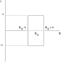
Figure 1: The cross section of the plasma boundary. The aspect ratio $\alpha$ is defined as $R_{0}/b$.

In addition, we assume that the plasma boundary coincides with the outermost magnetic surface; accordingly, the function $\psi$ should satisfy the following boundary conditions

$$\psi(y_{\pm})=0$$ (26)

and

$$\psi(x_{\pm})=0,$$ (27)

where $y_{\pm}=\pm\mbox{a}/R_{0}$ and $x_{\pm}=1\pm b/R_{0}$. The equilibrium becomes then a boundary-value problem. Eigenstates can be determined by imposing conditions (26) and (27) directly to solutions (23) and (25). Specifically, (26) applied to the $z$-dependent part of the solutions yields the eigenvalues

$$I_{1}^{\ell}=\frac{1}{\mbox{a}}\left(\ell\pi-\frac{\pi}{2}\right),\ \ \ell=1,2,\ldots$$ (28)

for the quantity $I_{1}$ which is related to the poloidal current function $I(\psi)$. The respective eigenfunctions are associated with configurations possessing $\ell$ magnetic axes parallel to the axis of symmetry. Condition (27) is pertinent to the $R$-dependent part of the solution. Owing to the flow this part contains the parameter $M_{0}$ in the compressible case and $A$ in the incompressible one in addition to the pressure parameter $P_{0}$. (To make further discussion easier we introduce the symbol $F$ representing either $M_{0}$ or $A$; this is particularly convenient to formulate results which are independent of ”compressibility”.) Thus, condition $\ref{25b})$ can determine eigenvalues depending on the parameter $P_{0}$ which remains free, $F^{n}(P_{0})$ ($n=1,2,3,\ldots$), or vice versa, pressure eigenvalues $P_{0}^{n}(F)$ with $F$ being free. This parametric dependence makes the spectrum of the eigenvalues broader in comparison with the static one. The eigenvalues depend also on the geometrical quantities $R_{0}$ and $b$ but not on a (see Fig. 1); thus, the results to follow are independent of elongation $\mbox{a}/b$. The other parameters $C_{1}$ and $C_{2}$ contained in (21) and (23) are adapted to normalize $\psi$ with respect to the magnetic axis and to satisfy the boundary condition (27) respectively. Also, in the rest of the report dimensionless values of $A$ will be given normalized with respect to 1 Kgr/(m⁷ T² s²). The eigenvalues $F^{n}(P_{0})$ and $P_{0}^{n}(F)$ can be calculated numerically. For a fixed value of $P_{0}$, $F^{n}$ satisfy for all $n$ the inequality $F^{n+1}>F^{n}$. A similar relation is satisfied by $P_{0}^{n}$ for a given value of $F$. The respective eigenfunctions are connected to configurations having $n$ magnetic axes perpendicular to the axis of symmetry. Therefore, the total equilibrium eigenfunctions $\psi_{\ell n}={\cal Z}_{\ell}(z){\cal R}_{n}(R)$ describe multitoroidal configurations having $\ell\times n$ magnetic axes. For example, a static doublet configuration, $\psi_{12}$, possessing two magnetic axes parallel to $z$-axis was studied in Ref. [11].

Henceforth, for the sake of simplicity we will restrict the study to eigenfunctions $\psi_{1n}$ describing multitoroidal configurations with $n$ magnetic axes along the mid-plane $z=0$. As an example the $\psi_{12}$-configuration for ”compressible” flow is shown in (Fig. 2).

\psfrag{R}{x}\psfrag{z}{y}\includegraphics[scale={0.8},trim=200.74998pt 100.37498pt 200.74998pt 100.37498pt]{2ndM.eps}

Figure 2: The double-magnetic-axis toroidal ”compressible” configuration in connection with the eigenfunction $\psi_{12}$ with eigenvalue $M_{0}^{2}=1.692$ for aspect ratio $\alpha=3$.

For vanishing flow, tokamak multitoroidal configurations of this kind were investigated in Ref. [2] in connection with hole current density profiles which can reverse in the core region; current reversal is possible because the configurations have non-nested magnetic surfaces. It is noted that for static equilibria only pressure eigenvalues are possible. In the presence of flow we examined eigenstates with the lowest of the pressure eigenvalues $P_{0}^{n}(F)$ by varying continuously the flow parameter $F$ starting from a value close to the first-order static one, $P_{0}^{1}(F\approx 0)$. It should be noted here that for incompressible flow, $A=0$ does not necessarily imply static equilibrium because of the non-zero shear [see Eq. (24)]. It turns out that there are transition points $F_{m}\ (m=1,2,\ldots)$ at which the configuration changes topology by the formation of an additional magnetic axis (The subscript $m$ here indicating a transition point must not be mixed up with the superscript $n$ indicating the order of an eigenvalue). For incompressible flow this is shown in Fig. 3.

\psfrag{R}{x}\psfrag{z}{y}\psfrag{a}{(a)}\psfrag{b}{(b)}\psfrag{c}{(c)}\psfrag{d}{(d)}\psfrag{e}{(e)}\psfrag{f}{(f)}\includegraphics[scale={1}]{seq.eps}

Figure 3: A sequence of graphs showing the quasi-static ”evolution” of the configuration as the incompressible flow parameter $A$ is decreased for aspect ratio $\alpha=3$. The values of $A$ for the individual plots are (a) $A=0.09$, (b) $A=-0.01$, (c) $A=-0.02$, (d) $A=-0.1$, (e) $A=-0.122$, (f) $A=-0.2$.

Specifically, the singly toroidal configuration 3(a) has eigenfunction $\psi_{11}$ with eigenvalue $P_{0}^{1}(A=0.09)$. By varying the flow parameter the pressure (eigenvalue) decreases and the configuration is shifted outwards and is compressed in the outer region while the pressure becomes lower (3(b)). Then, as the flow parameter reaches the first transition point $A_{1}=-0.01$ a second magnetic axis is formed in the outer region close to the boundary causing the first one to be shifted inwards (3(c)). This transition point is associated with pressure eigenvalue $P_{0}^{2}(A=A_{1})$. By a further increase of the flow (lower negative values of $A$) the outer magnetic island becomes bigger and the whole configuration is shifted outwards up to the next transition point $A_{2}=-0.1$ associated with pressure eigenvalue $P_{0}^{3}(A=A_{2})$ (Fig. 3(d)) at which as before a third magnetic axis is formed in the outer region; thus, the configuration consists of three magnetic islands (Fig. 3(e)) and is shifted outwards as the flow increases even more (Fig. 3(f)). This procedure is carried on until the formation of $n$ magnetic axes and it is also possible for ”compressible” flow. It can approximately be regarded as a quasi-static ”evolution” of the plasma due to the flow variation through flow-depended pressure equilibrium eigenstates. Therefore, it is not possible for static equilibria. An animation showing this ”evolution” is available in Ref [12]. Alternatively, varying continuously the pressure parameter $P_{0}$ one can find pressure transition points, $(P_{0})_{m}$, associated with flow eigenvalues.

For aspect ratio $\alpha=3$ and compressible flow the first transition velocity from a singlet to a doublet configuration is of the order of $10^{5}$ m/s. Velocities of this order have been measured in tokamaks and therefore the change in magnetic topology by the flow can be experimentally examined.

It is emphasized that the change of the magnetic topology due to the flow is not possible in the limit of infinite aspect ratio because in this limit the equilibrium equations do not contain the axial velocity regardless of ”compressibility”. Indeed, for a cylindrical plasma of arbitrary cross-section the equations respective to (15) and (16) read

$${\bf B}\cdot{\bf\nabla}P=0$$ (29)

$$\nabla^{2}\psi+\Big{(}P+\frac{B_{z}^{2}}{2}\Big{)}^{\prime}=0.$$ (30)

Eqs. (29) and (30) follow respectively from (16) and (17) of Ref [13] for vanishing poloidal velocity ($F^{\prime}=0$). Also, note that the pressure becomes a flux-function.

In addition, toroidicity affects qualitatively the eigenvalues and the transition points. We examined this impact by varying the aspect ratio $\alpha$ and found the following results:

1. The eigenvalues $P_{0}^{n}$ and $F^{n}$ (”compressible and incompressible) become lower as the aspect ratio decreases. For example, for $\alpha=3$ and $\alpha=2$ one finds $M_{0}^{2}=2.8$ and $M_{0}^{2}=2.3$, respectively.

2. The smaller $\alpha$ the lower the transition Mach numbers $(M_{0})_{m}$ and $A_{m}$ (for any $m$). For example, for $\alpha=3$ and $\alpha=2$ the respective first-transition Mach numbers are $(M_{0})_{1}=1.692$ and $(M_{0})_{1}=1.338$ and the first-transition incompressible points are $A_{1}=-0.083$ and $A_{1}=-0.448$.

The ”compressible” transition velocities are found to be in general supersonic. Experimental supersonic toroidal velocities have been reported in Refs. [14] and [15]. Owing to the above mentioned dependence of the transition points on $\alpha$, however, it is possible to have subsonic transitions for appropriate low values of $\alpha$. Thus, in this case the transitions may be realized easier in spherical tokamaks; the minimum subsonic value of the first-transition point $(M_{0})_{1}$ is 0.62 and corresponds to a compact toroid ($\alpha=1$).

IV. Shafranov shift

We evaluated the impact of the flow and the aspect ratio on the Shafranov shift of eigenstates with a single magnetic axis. (It is reminded that the Shafranov shift is defined as the displacement of the magnetic axis with respect to the geometrical center of the configuration, $\Delta x\equiv x_{m.a.}-1$.) The results are summarized as follows.

1. As $M_{0}$ increases or $A$ decreases the Shafranov shift increases. This increase for ”compressible and incompressible equilibria can be seen in Tables 1 and 2, respectively. It is interesting to note that for large positive values of $A$ the Shafranov shift can become negative. As an example for $\alpha=3$ and $A=0.09$ the shift is $-0.0274$. This means that the magnetic surfaces in this case are shifted inward. An inward shift of magnetic surfaces associated with poloidal flow in quasi-isodymanic equilibria was reported in Ref. [16]. Also, suppression of the Shafranov shift by a properly shaped toroidal rotation profile was found in Ref. [17].

   $M$	Shafranov Shift
   0.1	0.054
   0.4	0.058
   0.6	0.063

   Table 1: The Shafranov shift, $\Delta x\equiv x_{m.a.}-1$, for various values of the Mach number ($M_{0}$) and aspect ratio $\alpha=3$.

   A	Shafranov Shift
   0.010	0.045
   0.006	0.049
   -0.001	0.055

   Table 2: The Shafranov shift, $\Delta x\equiv x_{m.a.}-1$, for various values of the incompressible-flow parameter $A$ and aspect ratio $\alpha=3$.

2. The lower the aspect ratio the larger the Shafranov shift. This is shown in tables 3 and 4 for two different values of the pressure parameter $P_{0}$.

   Aspect ratio	Shafranov shift
   3	0.092
   2	0.150
   1.5	0.209

   Table 3: The Shafarnov shift, $\Delta x\equiv x_{m.a.}-1$, for $P_{0}=12$ kPa and various values of the aspect ratio for the ”compressible” case.

   Aspect ratio	Shafranov shift
   3	0.053
   2	0.140
   1	0.500

   Table 4: The Shafarnov shift, $\Delta x\equiv x_{m.a.}-1$, for $P_{0}=110$ kPa and various values of the aspect ratio for the incompressible case.

V. Summary and Conclusions

Equilibrium eigenstates of a magnetically confined plasma with toroidal flow surrounded by a boundary of rectangular cross-section have been investigated within the framework of ideal MHD theory. ”Compressible” flows associated with uniform temperature but varying density on magnetic surfaces and incompressible ones with uniform density but varying temperature thereon have been examined on the basis of respective reduced equations [(18) and (21)] and exact solutions [(23) and (25)]. The flow effect on the magnetic topology of the eigenstates has been examined by means of the parameters $M_{0}$ and $A$ associated with the quantities $\omega^{2}/T$ in the ”compressible” and $\varrho\omega^{2}$ in incompressible case, respectively. The exact ”compressible” solutions considered are shearless $[(\omega^{2}/(T))^{\prime}=0]$ while the incompressible ones have non-zero shear [$(\varrho\omega^{2})^{\prime}\neq 0$].

Owing to the flow one can consider either pressure eigenvalues, $(P_{0})^{n}\ n=1,2,\ldots$ with the flow parameter $F$ being free ($F$ represents either $M_{0}$ or $A$) or alternatively flow eigenvalues $F^{n}$ with free $P_{0}$. For fixed $F$ in the former case and fixed $P_{0}$ in the latter one, the eigenvalues satisfy the relations $P_{0}^{n+1}>P_{0}^{n}$ and $F^{n+1}>F^{n}$, respectively. The respective eigenfunctions for the poloidal magnetic flux-function $\psi$ can describe multitoroidal configurations with $n$ magnetic axes located on the mid-plane $z=0$. When $M_{0}$ is increased or $A$ is decreased continuously there are transition points $F_{m}$ ($m=1,2,\ldots$) at which an additional magnetic axis appears. Alternatively, by varying continuously the pressure parameter $P_{0}$ there are transition points $(P_{0})_{m}$ associated with flow eigenvalues at which an additional magnetic axis is formed. This change in magnetic topology, possible only in the presence of flow, is crucially related to toroidicity because in the limit of infinite aspect ratio the equilibrium equations are flow independent. The above mentioned ”flow-triggered” transitions can be approximately viewed as a quasi-static ”evolution” of the plasma by continuous flow variation through pressure eigenstates or alternatively by continuous pressure variation through flow eigenstates. The transition points have the following dependence on the aspect ratio $\alpha$: the lower $\alpha$ the smaller $(M_{0})_{m}$ in the ”compressible” case and $A_{m}$ in the incompressible one.

Also, we have examined the impact of the flow and the aspect ratio $\alpha$ (as a measure of the toroidicity) on the Shafranov shift. The results show that the shift (a) increases as $M_{0}$ take larger values and $A$ smaller ones and (b) increases as $\alpha$ takes lower values. Furthermore, for large positive values of $A$ the shift can become negative.

References

- [1] P. W. Terry, Rev. Mod. Phys. 72, 109 (2000).
- [2] A. A. Martynov, S. Yu. Medvedev, L. Villard, Phys. Rev. Lett. 91, 085004 (2003).
- [3] E. K. Maschke and H. Perrin, Plasma Phys. 22 579 (1980).
- [4] H. Tasso and G. N. Throumoulopoulos, Phys. Plasmas 5 2378 (1998).
- [5] R. A. Clemente and R. Farengo, Phys. Fluids 27 776 (1984).
- [6] G. N. Throumoulopoulos and G. Pantis, Phys. Fluids B 1, 1827 (1989).
- [7] Ch. Simintzis, G. N. Throumoulopoulos, G. Pantis, H. Tasso, Phys. Plasmas 8, 2641 (2001).
- [8] G. N. Throumoulopoulos, G. Poulipoulis, G. Pantis, H. Tasso, Phys. Lett. A 317, 463 (2003).
- [9] V. D. Shafranov, Rev. Plasma Phys. 2, 103 (1966).
- [10] L. S. Solovév, Rev. Plasma. Phys. 6, 239 (1976).
- [11] E. K. Maschke, Plasma Phys. 15, 535 (1973).
- [12] URL site: http://users.uoi.gr/me00584/plasma.htm .
- [13] G. N. Throumoulopoulos and H. Tasso, Phys. Plasmas 4, 1492 (1997).
- [14] L. R. Baylor et al, Phys. Plasmas 11, 3100 (2004).
- [15] L. Guazzotto, R. Betti, J. Manickam, S. Kaye, Phys. Plasmas 11, 604 (2004).
- [16] B. Hu, L. Guazzotto and R. Betti, Quasi-omnigenous tokamak equilibria with fast poloidal flow, 2004 International Sherwood Fusion Theory Conference, April 26-28, Missoula, Montana, USA; Abstract 1E48.
- [17] V. I. Il’gisonis, Yu. I. Pozdnyakov, JETP Lett. 71, 314 (2000).