Bound-state corrections in laser-induced nonsequential double ionization

Abstract

We perform a systematic analysis of how nonsequential double ionization in intense, linearly polarized laser fields is influenced by the initial states in which both electrons are bound, and by the residual ionic potential. We assume that the second electron is released by electron-impact ionization of the first electron with its parent ion, using an S-Matrix approach. We work within the Strong-Field Approximation, and compute differential electron momentum distributions using saddle-point methods. Specifically, we consider electrons in $1s$, $2p$, $3p$ and localized states, which are released by either a contact or a Coulomb-type interaction. We also perform an adequate treatment of the bound-state singularity which is present in this framework. We show that the momentum distributions are very sensitive with respect to spatially extended or localized wave functions, but are not considerably influenced by their shape. Furthermore, the modifications performed in order to overcome the bound-state singularity do not significantly alter the momentum distributions, apart from a minor suppression in the region of small momenta. The only radical changes occur if one employs effective form factors, which take into account the presence of the residual ion upon rescattering. If the ionic potential is of contact type, it outweighs the spreading caused by a long-range electron-electron interaction, or by spatially extended bound states. This leads to momentum distributions which exhibit a very good agreement with the existing experiments.

I Introduction

Within the last few years, nonsequential double ionization (NSDI) in strong, linearly polarized laser fields has attracted a great deal of attention, both experimentally and theoretically nsdireview . This interest has been triggered by the outcome of experiments in which the momentum component parallel to the laser field polarization could be resolved, either for the doubly charged ion expe1ion , or for both electrons expe1 . Indeed, the observed features, namely two circular regions along the parallel momenta $p_{1\parallel}=p_{2\parallel}$ peaked at $p_{1\parallel}=p_{2\parallel}=\pm 2\sqrt{U_{p}}$, with $U_{p}$ the ponderomotive energy, are a clear fingerprint of electron-electron correlation, and can be explained by a simple, three-step rescattering mechanism corkum . Thereby, an electron leaves an atom through tunneling ionization (the “first step”), propagates in the continuum, being accelerated by the field (the “second step”), and recollides inelastically with its parent ion (the “third step”). In this collision, it transfers part of its kinetic energy to a second electron, which is then released.

From the theoretical point of view, there exist models, both classical class ; slowdown ; pulse and quantum-mechanical abeckerrep ; abecker ; smatrix ; lphys ; pransdi1 ; pransdi2 ; pulseqm , based on such a mechanism, which qualitatively reproduce the above-mentioned features. They leave, however, several open questions. A very intriguing fact is that, for instance, a very good agreement with the experiments is obtained if the interaction through which the first electron is dislodged is of contact type, and if no Coulomb repulsion is taken into account in the final electron states. This agreement worsens if this interaction is modeled in a more refined way, considering either a more realistic, Coulomb-type interaction, or final-state electron-electron repulsion. Specifically, in recent publications, such effects have been investigated in detail using both an S-Matrix computation and a classical ensemble model, and have been interpreted in terms of phase-space and dynamical effects pransdi1 ; pransdi2 . This analysis has been performed within the Strong- Field Approximation (SFA) kfr , which mainly consists in neglecting the atomic binding potential in the propagation of the electron in the continuum, the laser field when the electron is bound or at the rescattering, and the internal structure of the atom in question.

Within this framework, the NSDI transition amplitude is written as a five-dimensional integral, with a time-dependent action and comparatively slowly varying prefactors. Such an integral is then solved using saddle-point methods. Apart from being less demanding than evaluating such an integral numerically abeckerrep ; abecker , or solving the time-dependent Schrödinger equation tdse , these methods provide a clear space-time picture of the physical process in question. In particular, the results are interpreted in terms of the so-called“quantum orbits”. Such orbits can be related to the orbits of classical electrons, and have been extensively used in the context of above-threshold ionization, high-order harmonic generation orbits and, more recently, nonsequential double ionization lphys ; pransdi1 ; pransdi2 ; pulseqm .

The fact that, in pransdi1 ; pransdi2 , the crudest approximation yields the best agreement with the experiments, seems to indicate that the presence of the residual ion, which is not taken into account, screens both the long-range interaction which frees the second electron and the final-state repulsion. This suggests that the presence of the ionic binding potential in the physical steps describing nonsequential double ionization, i.e., tunneling, propagation and electron-impact ionization, should somehow be incorporated. Indeed, in recent studies, it was found that Coulomb focusing considerably influences the NSDI yield coulombfocusing .

Another possibility is related to how the initial states in which the electrons are bound affect the electron-momentum distributions. Indeed, the poor agreement between the computations with the Coulomb interaction and the experiments may be related to the fact that 1s states have been used in this case, instead of states with a different shape or spatial symmetry, such as, for instance, p states. Furthermore, it may as well be that an additional approximation performed in pransdi1 ; pransdi2 for the contact interaction, namely to assume that it takes place at the origin of the coordinate system, contributes to the good agreement between theory and experiments in this case. Physically, this means that the spatial extension of the wave function of the second electron is neglected. Such an approximation has not been performed in the computations for the Coulomb interaction discussed in pransdi1 ; pransdi2 , and, up to the present date, there exist no systematic studies of its influence in the context of NSDI.

In this paper, we investigate such effects in the simplest possible ways. First, we assume that both electrons are initially in hydrogenic $2p$ and in $3p$ states, instead of in $s$ states, as previously done lphys ; pransdi1 ; pransdi2 ; pulseqm . One should note that, in contrast to Helium, for which $s$ states are more appropriate, $p$ states yield a more realistic description of the outer-shell electrons in neon and argon, respectively. Since the two latter species are used in most experiments, the choice of $p$ states is justified. This is included in the transition amplitude as a form factor, and does not modify the saddle-point equations. In both $p$ and $s$ - state cases, we consider that the bound-state wave function of the second electron is either localized at the origin or extends over a finite spatial range, for the contact and Coulomb interactions. This provides information on how the initial state of the second electron influences electron-impact ionization, and hence the NSDI yield.

A further improvement consists in overcoming the bound-state singularity, which is present in the saddle-point framework, and which has not been addressed in pransdi1 ; pransdi2 . For this purpose, we use a slightly modified action, with respect to that considered in pransdi1 ; pransdi2 , so that the tunneling process and the propagation of both electrons in the continuum is altered. Such corrections depend on the initial wave function of the first electron. Hence, they shed some light on how this wave function affects the electron-momentum distributions. In particular, we investigate how such corrections influence several features in the momentum distributions, such as their shapes, the cutoff energies or the contributions from different types of orbits to the yield.

Finally, we employ a modified form factor for the first electron, upon return, which takes into account the ionic potential. This is a first step towards incorporating the residual ion in our formalism. As it will be discussed subsequently, this provides a strong hint that the ion is important, in order to achieve a good agreement between theory and experiment.

The manuscript is organized as following. In Sec. II, we provide the necessary theoretical background for understanding the subsequent discussions. In Secs. III, IV, and V, we present our results, and, finally, in Sec. VI we state our conclusions.

II Background

II.1 Transition amplitude

The transition amplitude of the laser-assisted inelastic rescattering process responsible for NSDI, in the strong-field approximation and in atomic units, is given by

$$M=-\int_{-\infty}^{\infty}dt\int_{-\infty}^{t}dt^{\prime}\int d^{3}kV_{\mathbf{p}_{j}\mathbf{,k}}V_{\mathbf{k,}0}\exp[iS(t,t^{\prime},\mathbf{p}_{j},\mathbf{k})],$$ (1)

with the action

$$S(t,t^{\prime},\mathbf{p}_{j},\mathbf{k}) = -\frac{1}{2}\sum_{j=1}^{2}\int_{t}^{\infty}[\mathbf{p}_{j}+\mathbf{A}(\tau)]^{2}d\tau$$

$$-\frac{1}{2}\int_{t^{\prime}}^{t}[\mathbf{k}+\mathbf{A}(\tau)]^{2}d\tau+|E_{01}|t^{\prime}+|E_{02}|t.$$

Eq. (1) describes the following physical process: at a time $t^{\prime},$ both electrons are bound ($|E_{01}|$ and $|E_{02}|$ denote the first and second ionization potentials, respectively). Then, the first electron leaves the atom by tunneling ionization, and propagates in the continuum from the time $t^{\prime}$ to the time $t$, only under the influence of the external laser field $\mathbf{E}(t)=-d\mathbf{A}(t)/dt$. At this latter time, it returns to its parent with intermediate momentum $\mathbf{k}$, and gives part of its kinetic energy to the second electron through the interaction $V_{12}$, so that it is able to overcome the second ionization potential $|E_{02}|$. Finally, both electrons reach the detector with final momenta $\mathbf{p}_{j}$ $(j=1,2)$. All the influence of the binding potential $V$ and of the electron-electron interaction $V_{12}$ is included in the form factors

$$V_{\mathbf{p}_{j},\mathbf{k}}=<\mathbf{p}_{2}+\mathbf{A}(t),\mathbf{p}_{1}+\mathbf{A}(t)|V_{12}|\mathbf{k}+\mathbf{A}(t),\psi_{0}^{(2)}>$$ (3)

and

$$V_{\mathbf{k,}0}=<\mathbf{k}+\mathbf{A}(t^{\prime})|V|\psi_{0}^{(1)}>,$$ (4)

which are explicitly given by

$$V_{\mathbf{k,}0}=\frac{1}{(2\pi)^{3/2}}\int\!\!d^{3}r_{1}\exp[i(\mathbf{k}+\mathbf{A(}t^{\prime}\mathbf{)}).\mathbf{r}_{1}]V(\mathbf{r}_{1})\psi_{0}^{(1)}(\mathbf{r}_{1})$$ (5)

and

$$V_{\mathbf{p}_{j},\mathbf{k}} = \frac{1}{(2\pi)^{9/2}}\int\int d^{3}r_{1}d^{3}r_{2}\exp[i(\mathbf{p}_{1}-\mathbf{k}).\mathbf{r}_{1}]$$ (6)

$$\!\!\!\times\exp[i(\mathbf{p}_{2}+\mathbf{A(}t\mathbf{)}).\mathbf{r}_{2}]V_{12}(\mathbf{r}_{2},\mathbf{r}_{1})\psi_{0}^{(2)}(\mathbf{r}_{2}),$$

respectively. The binding potential $V(\mathbf{r}_{1})$ will be taken to be of Coulomb type, and the interaction $V_{12}(\mathbf{r}_{2},\mathbf{r}_{1})$ through which the second electron is released will be chosen to be of contact or Coulomb type. The initial state $\psi_{0}^{(1)}(\mathbf{r}_{1})$ of the first electron at the moment of its ionization will be taken as a hydrogenic $s$ or $p$ state, and the wave function $\psi_{0}^{(2)}(\mathbf{r}_{2})$ of the second electron at the moment of its release is either chosen as a hydrogenic state, or a Dirac delta state localized at $\mathbf{r}_{2}=0$. In Eq. (1), we neglect final-state electron-electron repulsion (for a discussion of this effect see Refs. abeckerrep ; pransdi2 ).

II.2 Saddle-point analysis

We solve Eq. (1) applying the steepest descent method, which is a very good approximation for low enough frequencies and high enough driving-field intensities. In this case, we must find $\mathbf{k}$, $t^{\prime}$ and $t$ so that $S(t,t^{\prime},\mathbf{p}_{n},\mathbf{k})$ $(n=1,2)$ is stationary, i.e., its partial derivatives with respect to these parameters vanish. This yields

$$\left[\mathbf{k}+\mathbf{A}(t^{\prime})\right]^{2}=-2|E_{01}|$$ (7)

$$\sum_{j=1}^{2}\left[\mathbf{p}_{j}+\mathbf{A}(t)\right]^{2}=\left[\mathbf{k}+\mathbf{A}(t)\right]^{2}-2|E_{02}|$$ (8)

$$\int_{t^{\prime}}^{t}d\tau\left[\mathbf{k}+\mathbf{A}(\tau)\right]=0.$$ (9)

Eq. (7) gives the energy conservation during tunneling ionization, and, for a non-vanishing ionization potential, has no real solution. Consequently, $t,t^{\prime}$ and $\mathbf{k}$ are complex quantities. In the limit $|E_{01}|\rightarrow 0,$ Eq. (7) describes a classical electron leaving the origin of the coordinate system with vanishing drift velocity. Eq. (8) expresses energy conservation at $t,$ in an inelastic rescattering process in which the first electron gives part of its kinetic energy to the second electron, so that it can overcome the second ionization potential and reach the continuum. Finally, Eq. (9) yields the intermediate electron momentum constrained by the condition that the first electron returns to the site of its release.

The saddles determined by Eqs. (7)-(9) always occur in pairs that nearly coalesce at the boundaries of the energy region for which electron-impact ionization is allowed to occur, within a classical framework. Such a boundary causes the yield to decay exponentially, leading to sharp cutoffs in the momentum distributions.

If written in terms of the momentum components parallel and perpendicular to the laser field polarization, Eq. (8) reads

$$\sum_{j=1}^{2}\left[p_{j||}+A(t)\right]^{2}=\left[\mathbf{k}+\mathbf{A}(t)\right]^{2}-2|E_{02}|-\sum_{j=1}^{2}\mathbf{p}_{j\perp}^{2}$$ (10)

and describes a hypersphere in the six-dimensional $(p_{j\parallel},\mathbf{p}_{j\perp})$ space. This hypersphere delimits a region in momentum space for which electron-impact ionization is “classically allowed”, i.e., exhibits a classical counterpart. For constant transverse momenta, Eq.  (10) corresponds to a circle in the $(p_{1||},p_{2||})$ plane centered at $-A(t)$ and whose radius is given by the difference between the kinetic energy $E_{\mathrm{kin}}(t)=1/2\left[\mathbf{k}+\mathbf{A}(t)\right]^{2}$ of the first electron upon return and the effective ionization potential $|\tilde{E}_{02}|=|E_{02}|+\sum_{j=1}^{2}\mathbf{p}_{j\perp}^{2}/2.$ Clearly, this radius is most extensive if the final transverse momenta $\mathbf{p}_{j\perp}),$ $(j=1,2)$ are vanishing, such as in the examples provided in Sec. IV.

In order to compute the transition probabilities, we employ a specific uniform saddle-point approximation, whose only applicability requirement is that the saddles occur in pairs Bleistein ; atiuni . Unless stated otherwise (e.g., in Sec. IV), we reduce the problem to two dimensions, using Eq. (9) and the fact that the action (II.1) is quadratic in $\mathbf{k}$. Details about this method, in the context of NSDI, are given in lphys ; pransdi1 ; pransdi2 ; pulseqm (for above-threshold ionization and high-order harmonic generation, c.f., atiuni and uniformhhg , respectively).

The momentum distributions of electrons for various types of interaction $V_{12}$ read

$$M=\int d^{2}p_{1\bot}\int d^{2}p_{2\bot}|M_{L}+M_{R}|^{2}$$ (11)

where the transverse momenta have been integrated over, and $M_{L}$ and $M_{R}$ give the left and the right peak in the momentum distributions, respectively, computed using the uniform approximation. We consider a monochromatic, linearly polarized field, so that the vector potential reads

$$\mathbf{A}(t)=-A_{0}\cos(\omega t)\mathbf{e}_{x}.$$ (12)

In this case, $M_{R}=M(t,t^{\prime},p)$ and $M_{L}=M(t-T/2,t^{\prime}-T/2,p),$ where $T=2\pi/\omega$ denotes a period of the driving field. We use the symmetry property $|M(t,t^{\prime},p)|=|M(t-T/2,t^{\prime}-T/2,-p)|$ to compute the left peak. One should note that, for other types of driving fields, such as few-cycle pulses, this condition does not hold and each peak must be computed independently pulse ; pulseqm .

III Initial p states

Within the formalism discussed in the previous section, the first and second electron, so far, have been assumed to be initially in $1s$- or zero-range-potential bound states, whose energies $|E_{01}|$ and $|E_{02}|$ are taken to be the first and second atomic ionization potential, respectively. In most experiments, however, species such as neon and argon are used, for which the outer-shell electrons are in $2p$ and $3p$ states, respectively. For this reason, such states should provide a more realistic modeling of laser-induced nonsequential double ionization. For symmetry reasons, only the states with magnetic quantum number $m=0$ will contribute to the yield.

In this case, the bound-state wave functions of both electrons will be given by

$$\psi_{210}^{(j)}(r_{j})=C_{210}r_{j}\exp[-\alpha_{j}r_{j}]\cos\theta$$ (13)

and

$$\psi_{310}^{(j)}(r_{j})=C_{310}r_{j}(1-\alpha_{j}r_{j}\ /2)\exp[-\alpha_{j}r_{j}]\cos\theta,$$ (14)

respectively, where $\alpha_{j}=\sqrt{2|E_{0j}|}(j=1,2)$, and $C_{n10}$ (where $n$ is the principal quantum number) denote normalization constants. For comparison, we will also consider hydrogenic $1s$ wave functions, which read

$$\psi_{100}^{\ (j)}(r_{j})=C_{100}\exp[-\alpha_{j}r_{j}].$$ (15)

In Eqs. (13)-(15),the binding energies of the first and the second electron were chosen as the first and the second ionization potentials, respectively.

The form factors $V_{\mathbf{p}_{j}\mathbf{,k}},$ for $2p$ and $3p$ initial states, read

$$V^{(2p)}_{\mathbf{p}_{j}\mathbf{,k}}\sim\eta(\mathbf{p}_{1},\mathbf{k})\frac{\tilde{p}}{\left[2|E_{02}|+\mathbf{\tilde{p}}^{2}\right]^{3}}+(\mathbf{p}_{1}\leftrightarrow\mathbf{p}_{2})$$ (16)

and

$$V^{(3p)}_{\mathbf{p}_{j}\mathbf{,k}}\sim\eta(\mathbf{p}_{1},\mathbf{k})\frac{\tilde{p}(\mathbf{\tilde{p}}^{2}-2|E_{02}|)}{\left[2|E_{02}|+\mathbf{\tilde{p}}^{2}\right]^{4}}+(\mathbf{p}_{1}\leftrightarrow\mathbf{p}_{2}),$$ (17)

respectively, with $\mathbf{\tilde{p}=p}_{1}+\mathbf{p}_{2}-\mathbf{k}+\mathbf{A}(t)$. Thereby, $(\mathbf{p}_{1}\leftrightarrow\mathbf{p}_{2})$ means that the momenta of both particles are interchanged, and $\eta(\mathbf{p}_{j},\mathbf{k})$ $(j=1,2)$ is a function which depends on the interaction in question. The corresponding form factor obtained for an initial state (15) is given by

$$V^{(1s)}_{\mathbf{p}_{j}\mathbf{,k}}\sim\eta(\mathbf{p}_{1},\mathbf{k})\frac{1}{\left[2|E_{02}|+\mathbf{\tilde{p}}^{2}\right]^{2}}+(\mathbf{p}_{1}\leftrightarrow\mathbf{p}_{2}).$$ (18)

III.1 Contact-type interaction

As a first step, we will assume that the second electron is released by a contact-type interaction

$$V_{12}\sim\delta(\mathbf{r}_{1}-\mathbf{r}_{2}).$$ (19)

In this case, in Eqs. (16)-(18), $\eta(\mathbf{p}_{j},\mathbf{k})$ is a constant. The differential electron momentum distributions computed with such form factors are depicted in Figs. 1(a)-1(c), as contour plots in the $(p_{1||},p_{2||})$ plane. In such computations, only the pair of orbits for which the electron excursion times $\tau=t-t^{\prime}$ in the continuum are shortest have been employed. As an overall feature, the distributions are peaked near $p_{1||}=p_{2||}=\pm\sqrt{U_{p}}$ and spread in the direction perpendicular to the diagonal $p_{1||}=p_{2||}$.

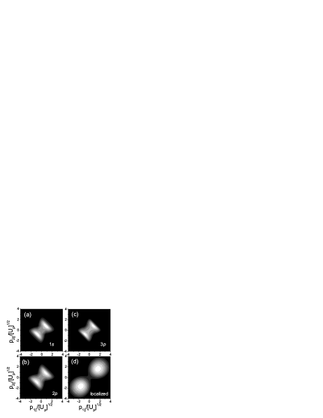
Figure 1: Electron momentum distributions computed using a contact-type interaction, as functions of the electron momentum components parallel to the laser-field polarization. The external field was taken to be monochromatic, with frequency $\omega=0.057$ a.u. and intensity $I=8\times 10^{14}\mathrm{W/cm}^{2}$ ($U_{p}=1.75$ a.u.). In panels (a), (b) and (c), both electrons are initially bound in a $1s$, $2p$, and $3p$ state [Eqs. (15), (13) and (14)], respectively, whereas, in part (d), the first electron is initially in a $1s$ state and the wave function of the second electron is localized at $r_{2}=0$. In all situations (even for the $3p$ - state case), the atomic species was taken to be neon ($|E_{01}|=0.79$ a.u. and $|E_{02}|=1.51$ a.u.), in order to facilitate a clear assessment of the effects caused by the different initial states. The transverse momenta have been integrated over.

An inspection of the form factors (16)-(18), for constant $\eta(\mathbf{p}_{j},\mathbf{k})$, explains this behavior. Indeed, such form factors are large if their denominator is small. Since $|E_{02}|$ is constant, this condition implies that $\mathbf{\tilde{p}=p}_{1}+\mathbf{p}_{2}-\mathbf{k}+\mathbf{A}(t)$ is small. To first approximation, since the first electron returns at times $t$ close to the minimum of the electric field, one may assume that the vector potential at this time and the intermediate electron momentum are approximately constant. Furthermore, in the model, the field is approximated by a monochromatic wave and $\mathbf{k}$ is given by Eq. (9). Hence, a rough estimate of these quantities at the return times yields $A(t)\simeq 2\sqrt{U_{p}}$ and $k\simeq 0$, respectively. Thus, $\mathbf{\tilde{p}}$ will be small mainly if $\mathbf{p}_{1}=-\mathbf{p}_{2}$, so that contributions along the anti-diagonal $p_{1||}=-p_{2||}$ will be enhanced.

Such contributions get more localized near the maxima for highly excited initial states due to the increase in the exponent of the denominator. A direct look at the above-stated form factors confirms this interpretation, yielding maxima along the anti-diagonal and near $\pm\sqrt{U_{p}}$.

Interestingly, the distributions obtained for the contact interaction are quite different from the circular distributions peaked around $p_{1||}=p_{2||}=\pm 2\sqrt{U_{p}}$ observed experimentally. Indeed, in order to obtain such distributions, it is necessary to assume that the initial wave function of the second electron is localized at $r_{2}=0.$ This is formally equivalent to taking

$$V_{12}(\mathbf{r}_{1}-\mathbf{r}_{2})\psi_{0}^{(2)}(\mathbf{r}_{2})\sim\delta(\mathbf{r}_{1}-\mathbf{r}_{2})\delta(\mathbf{r}_{2}).$$ (20)

Eq. (20) yields a constant form factor $V_{\mathbf{p}_{j},\mathbf{k}}$. In Fig. 1.(d), we present the distributions computed using Eq. (20), which exhibit a very good agreement with the experiments. This means that, in reality, the effective wave function of the second electron is very localized, most probably due to refocussing coulombfocusing , or screening effects footnscreening .

III.2 Coulomb-type interaction

We will now consider that the second electron is released by a Coulomb type interaction, given by

$$V_{12}=1/|\mathbf{r}_{1}-\mathbf{r}_{2}|.$$ (21)

In this case, in the form factors (16)-(18), $\eta$ is given by

$$\eta(\mathbf{p}_{j},\mathbf{k})=\frac{1}{[\mathbf{p}_{j}-\mathbf{k}]^{2}}\hskip 14.22636pt(j=1,2),$$ (22)

respectively. This causes the prefactors to be large when $\mathbf{p}_{j}-\mathbf{k}$ $(j=1,2)$ is small, in addition to the case for which $\mathbf{\tilde{p}}\ll 1$. The influence of such form factors on the electron momentum distributions is shown in Fig. 2. Apart from the broadening along $p_{1||}=-p_{2||}$ caused by the spatial extent of the bound-state wave functions (c.f. Sec. III.1), the distributions exhibit maxima near the axis $p_{1||}=0$ or $p_{2||}=0.$ Such maxima are due to the factor (22) in Eqs. (16)-(18), characteristic of the Coulomb-type interaction, which is large for $\mathbf{p}_{j}\simeq\mathbf{k}$. Since, to first approximation, contributions from regions of small $k$ dominate the yield, one expects maxima in momentum regions where either $\mathbf{p}_{1}$ or $\mathbf{p}_{2}$ are small.

Furthermore, as compared to the yields obtained using a Coulomb-type interaction and $1s$-states, there exists a small additional broadening in the distributions, with respect to the diagonal $p_{1||}=p_{2||}$, as well as an increase in the contributions from regions where such momenta are small. Such effects get more pronounced as the principal quantum number increases, as shown in Figs. 2.(b) and 2.(c).

However, such modifications do not alter the distributions in a significant way. More extreme changes occur, for instance, if a contact-type interaction, i.e., $\eta(\mathbf{p}_{j},\mathbf{k})=const.$ in Eq. (19), is taken into account. Still, less localized bound states for both electrons will cause a broadening in the momentum distributions. If the second-electron wave function is localized at the origin, the form factor (18) reduces to

$$V_{\mathbf{p}_{j}\mathbf{,k}}\sim\frac{1}{[\mathbf{p}_{1}-\mathbf{k}]^{2}}+(\mathbf{p}_{1}\leftrightarrow\mathbf{p}_{2}).$$ (23)

The distributions for the latter form factor are displayed in Fig. 2.(d). In the figure, one observes a considerable reduction of the broadening along the anti-diagonal $p_{1||}=-p_{2||}$. However, the distributions still exhibit the two sets of maxima near the axis $p_{1||}=0$ or $p_{2||}=0.$ This is expected, since such maxima are a fingerprint of the Coulomb interaction.

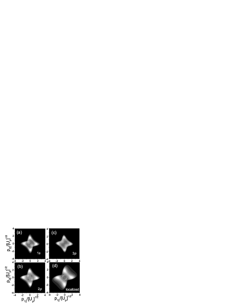
Figure 2: Electron momentum distributions computed using a Coulomb-type interaction, as functions of the electron momentum components parallel to the laser-field polarization. The field and atomic parameters are the same as in Fig. 1. In panels (a), (b) and (c), both electrons are taken to be initially in a $1s$, $2p$, and $3p$ state, respectively, whereas in panel (d) the first electron is in a $1s$ state, while the spatial extension of the bound-state wave function has been neglected. The transverse momenta have been integrated over.

The results in this section show that the shapes of the momentum distributions in NSDI are not only influenced by the type of interaction by which the second electron is dislodged but, additionally, depend on the spatial extension of the wave function of the state where it is initially bound. In fact, radically different shapes are observed if this wave function is either taken to be localized at $\mathbf{r}_{2}=0$ or exponentially decaying. This is true both for a contact- and a Coulomb-type interaction (c.f. Figs. 1.(d) and 2.(d)).

On the other hand, if different initial states are taken, for the same type of interaction, there are no significant changes in the shapes of the distributions as long as such states extend over a finite spatial range. This is explicitly seen by comparing yields obtained using bound states with different principal quantum numbers. This is related to the fact that the wave functions (13)-(15) were chosen such that the bound-state energy always corresponds to the second ionization potential. Hence, even if their shape changes, the spatial extension of such wave functions is roughly the same.

It is still, however, quite puzzling that the best agreement with the experimental findings occurs for the crudest approximations, both for the interaction and the initial bound-state wave function, i.e., for a contact-type interaction and a wave function localized at $\mathbf{r}_{2}=0.$ Indeed, taking either a more realistic type of electron-electron interaction, spatially extended bound states, or, still, bound states which are, in principle, a more refined description of the outer-shell electrons, only worsens the agreement between experiment and theory.

If the main physical mechanism of NSDI is electron-impact ionization, there exist two main possibilities for explaining this discrepancy. Either the second electron is bound in a highly localized state and both electrons collide through an effective short-range interaction, as the present results suggest, or the tunneling ionization, as well as the electron propagation in the continuum, must be improved. The first issue may be addressed by including the influence of the residual ion in the process, whereas the second issue may be dealt with in several ways. For instance, in the subsequent section, we will consider corrections of a more fundamental nature, which alter the semiclassical action and thus the orbits of the electrons.

IV Treatment of the bound-state singularity

Up to the present section, we have implicitly assumed that the form factors $V_{\mathbf{p}_{{j}}\mathbf{,k}}$ and $V_{\mathbf{k,}0}$ are free of singularities and slowly varying in comparison to the time-dependent action. However, this is not always true. Indeed, in the saddle-point framework, the form factor $V_{\mathbf{k,}0}$ is singular if the electron is initially in a state described by an exponentially decaying wave function, such as Eqs. (13)-(15). More specifically, in this case,

$$V_{\mathbf{k,}0}\varpropto\frac{f(k+A(t^{\prime}))}{\left(\left[\mathbf{k}+\mathbf{A}(t^{\prime})\right]^{2}+2|E_{01}|\right)^{n}},$$ (24)

where $n$ is an integer number. In this case, according to Eq. (7), the denominator vanishes. Due to this singularity, this form factor does not vary slowly with respect to the semi-classical action (II.1), and thus must be incorporated in the exponent. Therefore, we take the modified action

$$\tilde{S}(t,t^{\prime},\mathbf{p}_{j},\mathbf{k})=S(t,t^{\prime},\mathbf{p}_{j},\mathbf{k})-i\ln\left[V_{\mathbf{k,}0}\right]$$ (25)

in the transition amplitude (1). This causes a change in the first and third saddle-point equations, which will depend on the initial bound state in question. In particular, we will consider that the first electron is initially in the hydrogenic states $1s$, $2p$, and $3p$. This is a legitimate assumption, since the binding potential of a neutral atom, from which the first electron tunnels out, is of long-range type. For the states $1s$, $2p$, and $3p$, $V_{\mathbf{k},0}$ reads

$$V_{\mathbf{k},0}^{(1s)}=\frac{\sqrt{2}}{\pi}\frac{(2|E_{01}|)^{5/2}}{\mathbf{v}^{2}+2|E_{01}|},$$ (26)

$$V_{\mathbf{k},0}^{(2p)}=\frac{2\sqrt{2}i}{\pi}\frac{(\sqrt{2|E_{01}|})^{5/2}v}{(\mathbf{v}^{2}+2|E_{01}|)^{2}},$$ (27)

and

$$V_{\mathbf{k,}0}^{(3p)}=\frac{8i(\sqrt{2|E_{01}|})^{5/2}v(\mathbf{v}^{2}-2|E_{01}|)}{\sqrt{3}\pi(\mathbf{v}^{2}+2|E_{01}|)^{3}},$$ (28)

respectively, where $\mathbf{v}=\left[\mathbf{k}+\mathbf{A}(t^{\prime})\right]$ denotes the initial electron drift velocity. The explicit expressions for the saddle point equations then become

$$\left[\mathbf{k}+\mathbf{A}(t^{\prime})\right]^{2}=-2|E_{01}|+\mathbf{\zeta}(k,t^{\prime}).\mathbf{E}(t^{\prime})$$ (29)

and

$$\int_{t^{\prime}}^{t}d\tau\left[\mathbf{k}+\mathbf{A}(\tau)\right]+\mathbf{\zeta}(k,t^{\prime})=0,$$ (30)

respectively, where $\mathbf{\zeta}(k,t^{\prime})=-i\partial_{\mathbf{k}}\ln[V_{\mathbf{k,}0}]$ is a correction which depends on the initial bound state. Thus, there is an effective shift in the ionization potential at the tunneling times, and a modification in the return condition. Consequently, the orbits change. Apart from that, from the technical point of view, the transition amplitude is no longer reducible to a two-dimensional integral, so that the problem is far more cumbersome.

The modifications in the equation describing tunneling ionization allow the existence of solutions for which $\mathrm{Re}[v]\neq 0$. This did not occur in Eq. (7), for which this quantity was purely imaginary, and, physically, means that there are in principle changes, maybe even enhancements, in the probability that the first electron tunnels out at $t^{\prime}.$

Furthermore, Eq. (30), if written in terms of the components of the intermediate momentum $\mathbf{k}$ parallel and perpendicular to the laser field polarization, has, apart from the trivial solution $\mathbf{k}_{\perp}=0,$ additional solutions for which $\mathbf{k}_{\perp}\neq 0.$ Thus, in principle, the first electron may have, during the tunnel ionization and upon return, a non-vanishing drift velocity component transverse to the laser-field polarization. We regard this possibility, however, as non-physical, and therefore will mainly concentrate on the case of vanishing $\mathbf{k}_{\perp}.$ Despite of that, the results obtained for nonvanishing $\mathbf{k}_{\perp}$will be briefly discussed in Sec. IV.2. For the return condition (8) this is not possible and $\mathbf{k}_{\perp}$ is always vanishing. In the following, we will investigate how the corrections in the action affect the momentum distributions.

IV.1 Vanishing $\mathbf{k}_{\perp}$

In this section, we will consider that the first electron has vanishing intermediate momentum components $\mathbf{k}_{\perp}$. Physically, this means that the dynamics of NSDI is mainly taking place along the laser field polarization, which is the intuitively expected situation. In Fig. 3, we present the electron momentum distributions computed employing the modified saddle-point equations and the action (25), for the same initial states and types of as in Figs. 1 and a contact-type interaction. In general, the distributions in Fig. 3 are very similar to the former ones, with, however, a suppression in the region of small parallel momenta. This is true even if different corrections are taken into account, as it is the case if the first electron is initially in a $1s$, $2p$ and $3p$ state (Figs. 3.(a), 3.(b) and 3.(c), respectively). In the specific case of a localized bound-state wave function for the second electron, there is also a minor displacement of the maxima towards smaller parallel momenta(c.f. Fig. 3(d)).

The suppression persists if the second electron is released by a Coulomb-type interaction, as shown in Fig. 4. Specifically for this interaction, the corrections lead to a suppression of the secondary maxima in the small-momentum region, which were present in Fig. 2.

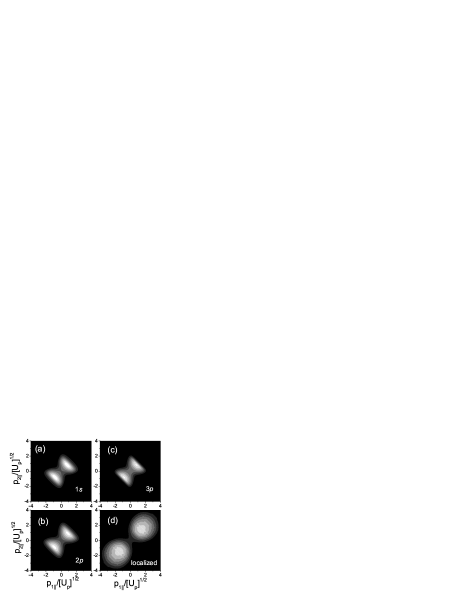
Figure 3: Electron momentum distributions computed with using contact-type interaction, as functions of the electron momentum components parallel to the laser-field polarization, for the same field and atomic parameters as in the previous figures. We introduce corrections to the bound-state singularity by employing the modified action (25) and saddle-point equations, taking the solutions displayed in Figs. 6.(a) and 6.(c). In panels (a), (b) and (c), both electrons are taken to be initially in a $1s$, in a $2p$, and in a $3p$ state, respectively, whereas in panel (d) the first electron is initially in a 1s state, while the spatial extension of the bound-state wave function of the second electron has been neglected. The transverse momenta have been integrated over.

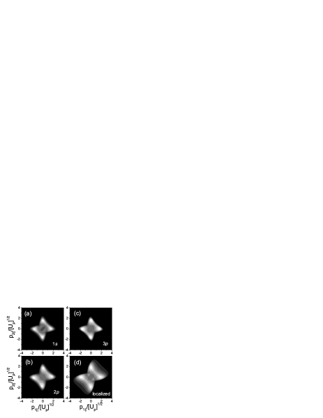
Figure 4: Electron momentum distributions computed using the Coulomb-type interaction, as functions of the electron momentum components parallel to the laser-field polarization, for same field and atomic parameters as in the previous figure. We introduce corrections to the bound-state singularity by employing the modified action (25) and saddle-point equations, and the solutions in Figs. 6(a) and 6.(c). In panels (a), (b) and (c), both electrons are taken to be initially in a $1s$, in a $2p$, and in a $3p$ state, respectively, whereas in panel (d) the first electron is initially in a 1s state, while the spatial extension of the bound-state wave function of the second electron has been neglected. The transverse momenta have been integrated over.

In the following, we will analyze these differences in terms of the so-called quantum orbits, obtained by solving the saddle point equations. We will consider both the saddle-point equations in the presence and absence of corrections to the bound-state singularity, i.e., Eqs. (29), (8) and (30), and (7)-(9), respectively. We restrict ourselves to vanishing final transverse momenta and longitudinal momentum components along the diagonal $p_{||}=p_{1||}=p_{2||}$. For this particular case, the energy region for which electron-impact ionization is classically allowed is most extensive.

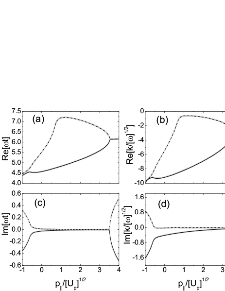
Figure 5: Rescattering times, together with the intermediate momentum $k_{||}$, as functions of the parallel momentum $p_{||}$ along the diagonal $p_{1||}=p_{2||}$. The final transverse momenta $\mathbf{p}_{j\perp}(j=1,2)$ and the intermediate transverse momentum $\mathbf{k}_{\perp}$ are taken to be vanishing. The real and imaginary parts of such quantities are displayed in the upper [(a), (b) and (c)] and lower [(d), (e) and (f)] panels, respectively. The field and atomic parameters are the same as in the previous figure.  The uncorrected variables are given by the thick light gray curves in the figure, while the variables with corrections corresponding  to initial $1s$, $2p$ and $3p$ states are given by the gray, dark gray and black curves, respectively. The longer and the shorter orbit are indicated by dashed and solid lines, respectively.

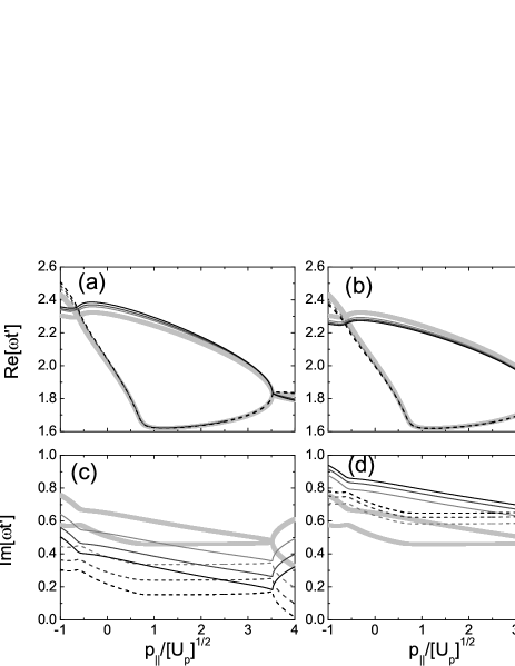
Figure 6: Tunneling times as functions of the parallel momentum $p_{||}$ along the diagonal $p_{1||}=p_{2||}$. The final transverse momenta $\mathbf{p}_{j\perp}(j=1,2)$ and the intermediate transverse momentum $\mathbf{k}_{\perp}$ are taken to be vanishing. The real and imaginary parts of such quantities are displayed in the upper [(a) and (b)] and lower [(c) and (d)] panels, and the same pairs of orbits are depicted in the left [(a) and (c)] and right [(b) and (d)] panels, respectively. The field and atomic parameters are the same as in the previous figure.  The uncorrected variables are given by the thick light gray curves in the figure, while the variables with corrections corresponding  to initial $1s$, $2p$ and $3p$ states are given by the gray, dark gray and black curves, respectively. The longer and the shorter orbit are indicated by dashed and solid lines, respectively.

In Fig. 5, we display the solutions of the saddle-point equations for the rescattering times $t$ and the intermediate momentum $\mathbf{k}$. The upper and lower panels in the figure give the real and imaginary parts of such variables, respectively. The real parts of $t$ and $\mathbf{k}$ correspond to the solutions of the equations of motion of a classical electron in an external laser field, and almost merge at two distinct parallel momenta. These momenta are related to the maximal and minimal energy for which the second electron is able to overcome $|E_{02}|.$ Beyond such momenta, there are cutoffs in the distributions, and the yield decays exponentially. The imaginary parts of such variables are in a sense a measure of a particular physical process being classically allowed or forbidden. Indeed, the fact that $|\mathrm{Im}[t]|$ and $|\mathrm{Im}[k]|$ are vanishingly small between the minimal and maximal allowed momenta are a consequence of both electron-impact ionization and the return condition being classically allowed in this region. As the boundaries of this region are reached, $|\mathrm{Im}[t]|$ and $|\mathrm{Im}[k]|$ increase exponentially. Interestingly, both the real and imaginary parts of such variables, as well as the cutoff momenta, remain practically inaltered upon the changes introduced in this section. This is not obvious, since the bound-state corrections in question alter the return condition [c.f. Eq.(30)].

There exist, however, modifications in the tunneling times $t^{\prime}$, which are explicitly shown in Fig. 6. Specifically, the corrections in the tunneling condition, which leads to Eq. (29), cause a splitting in the solutions of Eq. (7). This follows from the fact that small variations in the stationary-action trajectories contributes quadratically to $S(t,t^{\prime},\mathbf{p}_{j},\mathbf{k})$ and $V_{\mathbf{k},0}$, so that $\tilde{S}(t,t^{\prime},\mathbf{p}_{j},\mathbf{k})$ attains two stationary trajectories for each of the former ones. Strictly speaking, a similar splitting also occurs for $\mathbf{k}$ and $t$. In practice, however, the difference between the two different sets of solutions is vanishingly small, and thus not noticeable in Fig. 5. The different sets of solutions are depicted in Figs. 6(a) and 6.(c), and 6.(b) and 6(d), respectively.  The real parts $\mathrm{Re}[t^{\prime}]$ exhibit only minor differences, with occur for the shorter orbits and small momenta and eventually disappear as the upper cutoff is approached. Depending on the type of correction, such times either distance themselves from, or become slightly closer to the peak-field times (Figs. 6.(a) and 6.(b), respectively). Thus, one could expect an enhancement in the contributions from the shorter orbits near the origin of the $\left(p_{1||},p_{2||}\right)$ plane, in the former case, and a suppression in the latter case. However, we have used the solutions in Fig. 6.(b) and (d) for computing the contour plots in Figs. 3 and 4, and obtained a suppression in the yield. This is a clear indication that the changes in $\mathrm{Im}[t^{\prime}]$ and in the time-dependent action play a more important role than those in $\mathrm{Re}[t^{\prime}]$.

In Figs. 6.(c) and 6.(d), we present the imaginary parts of $t^{\prime},$ which clearly shift towards smaller, and larger values, respectively, when the corrections $\mathbf{\varsigma}(k,t^{\prime})$ are taken into account. The higher the initial state lies, the larger such shifts are. Physically, there exists a correspondence between such imaginary parts and the probability that the first electron tunnels out and reaches the continuum. This means that, by using a slightly modified action in order to overcome the Coulomb singularity, one is changing the effective potential barrier at $t^{\prime}$ for the first electron. In general, such a barrier has a significant influence on the distributions. Indeed, recently, we have shown, within the context of nonsequential double ionization with few-cycle laser pulses, that the importance of the contributions of a particular orbit or set of orbits to the yield is highly dependent on $|\mathrm{Im}[t^{\prime}]|$. The smaller this quantity is, the larger is the tunneling probability for the first electron pulseqm . As a direct consequence, contributions from orbits with small $|\mathrm{Im}[t^{\prime}]|$, i.e., with a large tunneling probability, dominate the yield. In the present case, however, since both orbits are being equally shifted, this should not influence the distributions qualitatively. One should note that, even in the momentum region for which electron-impact ionization is allowed, $|\mathrm{Im}[t^{\prime}]|$ is always nonvanishing. This is a direct consequence of the fact that tunneling ionization is a classically forbidden process.

Subsequently, we compute the counterparts of Fig. 3 and 4 (Figs. 7 and 8) using the solutions displayed in Fig. 6.(b) and 6.(d). Also in this case, in general, there is a suppression in the yield in the region of small parallel momenta, with, however, a slightly different substructure in the Coulomb-interaction case.

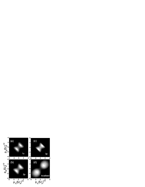
Figure 7: Electron momentum distributions computed with the contact-type interaction, as functions of the electron momentum components parallel to the laser-field polarization, for the same field and atomic parameters as in the previous figure. We introduce corrections to the bound-state singularity by employing the modified action (25) and saddle-point equations, taking the solutions in Figs. 6.(b) and 6.(d). In panels (a), (b) and (c), both electrons are taken to be initially in a $1s$, in a $2p$, and in a $3p$ state, respectively, whereas in panel (d) the first electron is in a $1s$ state, and spatial extension of the bound-state wave function of the second electron has been neglected. The transverse momenta have been integrated over.

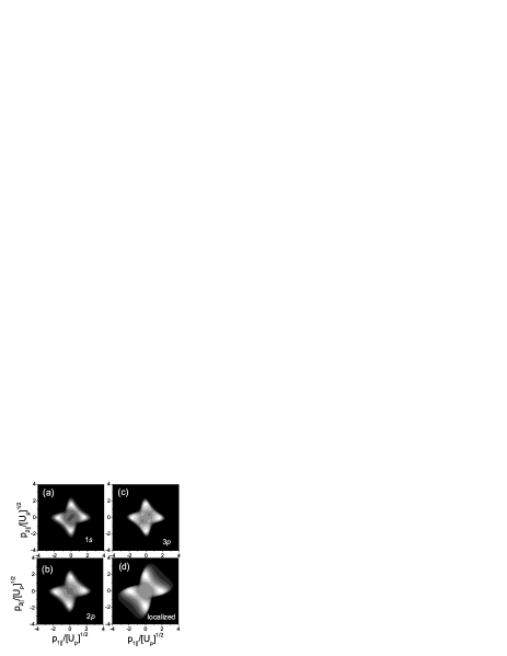
Figure 8: Electron momentum distributions computed using the Coulomb-type interaction, as functions of the electron momentum components parallel to the laser-field polarization, for same field and atomic parameters as in the previous figure. We introduce corrections to the bound-state singularity by employing the modified action (25) and saddle-point equations, and the solutions in Figs. 6.(b) and 6.(d). In panels (a), (b) and (c), both electrons are taken to be initially in a $1s$, in a $2p$, and in a $3p$ state, respectively, whereas in panel (d) the first electron is initially in a 1s state, while the spatial extension of the bound-state wave function of the second electron has been neglected. The transverse momenta have been integrated over.

IV.2 Nonvanishing $\mathbf{k}_{\perp}$

The modifications introduced in the return condition for the first electron [Eq. (30)] allow the intermediate momentum $\mathbf{k}$ to have a nonvanishing component perpendicular to the laser-field polarization.  This implies that the first electron, during tunneling ionization and when it returns, is being deviated from its original direction. Although such an effect is unphysical, we will briefly discuss its consequences.  For that purpose, we will consider the simplest corrections to the bound-state singularity discussed in this paper, namely those for $1s$ initial states. If Eq. (30) is written in terms of the intermediate-momentum components $\mathbf{k}_{\perp}$ and $k_{||}$ perpendicular and parallel to the laser-field polarization, this equation reads

$$k_{||}(t-t^{\prime})-\int_{t^{\prime}}^{t}A(s)ds+\frac{2i[k_{||}+A(t^{\prime})]}{\left[2|E_{01}|+\mathbf{k}_{\perp}^{2}+[k_{||}+A(t^{\prime})]^{2}\right]}=0$$ (31)

and

$$\mathbf{k}_{\perp}^{2}\left(t-t^{\prime}+\frac{2i}{\left[2|E_{01}|+\mathbf{k}_{\perp}^{2}+[k_{||}+A(t^{\prime})]^{2}\right]}\right)=0,$$ (32)

respectively. Apart from the trivial solution $\mathbf{k}_{\perp}=0,$ the condition (32) can be satisfied by nonvanishing values of this variable. One should note that, in the case without corrections, this does not hold and only the trivial solution exists.

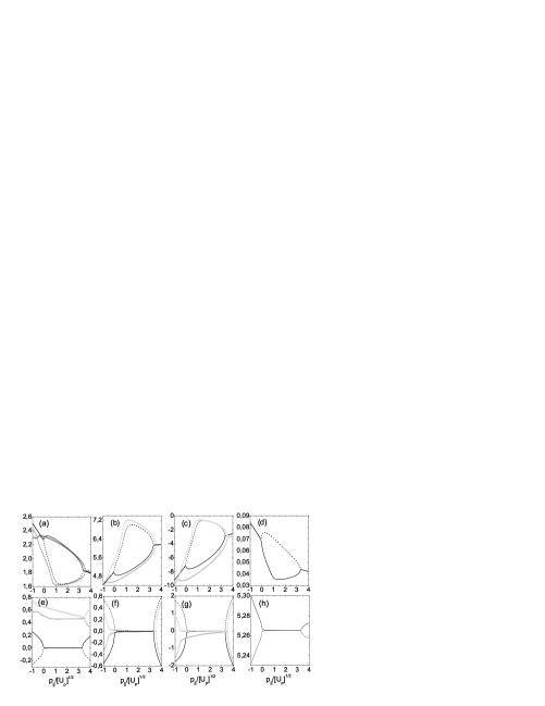
Figure 9: Tunneling [Panels (a) and (e)] and rescattering times [Panels (b) and (f)], together with the parallel [Panels (c) and (g)] and perpendicular components of the intermediate momentum $\mathbf{k}$ [Panels (d) and (h)], as functions of the parallel momentum $p_{||}$ along the diagonal $p_{1||}=p_{2||}$. The final transverse momenta $\mathbf{p}_{j\perp}(j=1,2)$ are taken to be vanishing. The real and imaginary parts of such quantities are displayed in the upper [(a), (b), (c) and (d)] and lower [(e), (f), (g) and (h)] panels, respectively. The field and atomic parameters are the same as in the previous figure. The corrected and uncorrected yields are given by the black and gray curves in the figure, respectively. The tunneling and rescattering times are multiplied by $\omega$ and the intermediate momenta divided by $\sqrt{\omega}$, respectively, so that a direct comparison with Figs. 5 and 6 can be performed.

Fig. 9 depicts the tunneling and rescattering times for this case, together with the perpendicular and parallel components of $\mathbf{k.}$ The real parts of such variables correspond, as in the previous cases, to a longer and a shorter orbit. The momenta, however, for which such orbits nearly coalesce, are radically different from those in the previous cases discussed in this paper. This is due to the fact that a nonvanishing $\mathbf{k}_{\perp}$ also affects the rescattering condition (8), which now reads

$$\sum_{j=1}^{2}\left[p_{j||}+A(t)\right]^{2}=\left[k_{||}+A(t)\right]^{2}+\mathbf{k}_{\perp}^{2}-2|E_{02}|-\sum_{j=1}^{2}\mathbf{p}_{j\perp}^{2}$$

For constant final transverse momenta $\mathbf{p}_{j\perp}(j=1,2),$ this equation describes a circle centered at $-A(t)$ whose radius has been altered in $\mathbf{k}_{\perp}^{2}$. Since, as shown in Figs 9(a)-9(d), this radius decreased, $\mathbf{k}_{\perp}$ is expected to be almost purely imaginary. This is indeed the case, as can be seen comparing panels (d) and (h) in the figure. The imaginary parts of such variables also behave following the same pattern as previously, growing vary rapidly at the momenta for which the real parts approach each other, and remaining nearly constant in-between. Interestingly, $\mathrm{Im}[t^{\prime}]$ is vanishing in this region. This feature is in clear contradiction with the fact that tunneling is a process which is always forbidden, and therefore requires a nonvanishing $\mathrm{Im}[t^{\prime}]$ (c.f. Fig. 5.(d)). For this reason, we will not use solutions with nonvanishing $\mathbf{k}_{\perp}$ for computing electron momentum distributions.

V Influence of the ion

In this section, we take a first step towards including the residual ion in our formalism. For that purpose, we consider an effective interaction $\widetilde{V}=V_{12}+V_{\mathrm{ion}}$ at the time the first electron returns, where $V_{\mathrm{ion}}$ is the ionic potential. Physically, this means that the first electron interacts not only with the electron it releases, but, additionally, with the residual ion. We take this potential to be of either Coulomb or contact type, and assume that only the two active electrons contribute to the ionic charge. Thus, explicitly,$V_{\mathrm{ion}}$ reads

$$V^{(C)}_{\mathrm{ion}}=-2/|\mathbf{r}_{1}|$$ (33)

or

$$V^{(\delta)}_{\mathrm{ion}}\sim-2\delta(\mathbf{r}_{1}).$$ (34)

In this context, both the effective charge and a contact-type interaction are justified by the fact that the remaining electrons are screening the charge and the long-range tail of the binding potential.

In Eq. (1), the form factors $V_{\mathbf{p_{j}},\mathbf{k}}$ are given by

$$\widetilde{V}^{(1s)}_{\mathbf{p}_{j},\mathbf{k}}\sim V^{(1s)}_{\mathbf{p}_{j},\mathbf{k}}-\frac{2\eta(\mathbf{p}_{1},\mathbf{k})}{[2|E_{02}|+(\mathbf{p}_{2}+\mathbf{A}(t))^{2}]^{2}}\newline +(\mathbf{p}_{1}\leftrightarrow\mathbf{p}_{2}),$$ (35)

$$\widetilde{V}^{(2p)}_{\mathbf{p}_{j},\mathbf{k}}\sim V^{(2p)}_{\mathbf{p}_{j},\mathbf{k}}-\frac{2\eta(\mathbf{p}_{1},\mathbf{k})\sqrt{(\mathbf{p}_{2}+\mathbf{A}(t))^{2}}}{[2|E_{02}|+(\mathbf{p}_{2}+\mathbf{A}(t))^{2}]^{3}}\newline +(\mathbf{p}_{1}\leftrightarrow\mathbf{p}_{2}),$$ (36)

for $1s$ and $2p$ states, respectively. The prefactor $V_{12}$ is of contact or Coulomb type. Furthermore, for a Coulomb or contact ionic potential, $\eta$ is either constant or given by Eq. (22), respectively. In order to simplify the computations, and since only minor differences have been observed in this case, we use the model in Sec. II, instead of the more rigorous approach of Sec. IV in the subsequent figures.

Fig. 10 depicts how the ion affects the electron momentum distributions, if its potential is assumed to be of Coulomb form (Eq.(33)). The upper and lower panels have been computed for $V_{12}$ of contact and Coulomb type, respectively. In the figure, the distributions resemble those obtained for the Coulomb-type interaction, if the second state is in a localized state (Figs. 2.(d), 4.(d), and 8.(d)). This holds both for $1s$ and $2p$ initial electron states. An inspection of Eqs. (35) and (36) explains this shape. Indeed, in both equations, the functional form of $\eta(\mathbf{p}_{j},\mathbf{k})$, which is characteristic of long-range interactions, favors unequal momenta, leading to patterns similar to those observed in Figs. 2, 4, and 8. Furthermore, in the second terms in $\widetilde{V}_{\mathbf{p}_{j},\mathbf{k}}$, the denominators are small if $\mathbf{p}_{j}\simeq-\mathbf{A}(t)$. Thus, since, $A(t)\sim 2\sqrt{U_{p}}$, we expect the form factors (35) and (36) to be large near $p_{2||}=p_{1||}=\pm 2\sqrt{U_{p}}$. Consequently, the yield in the diagonal gets enhanced. This is a feature shared with the limit for localized wave functions, so that the distributions are similar.

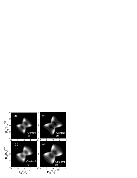
Figure 10: Electron momentum distributions computed with the modified form factors (35),(36), as functions of the electron momentum components parallel to the laser-field polarization, for same field and atomic parameters as in the previous figures. We consider that the ionic potential is of Coulomb type (Eq. (33)), and use the saddle-point model without modifications (c.f. Sec. II). In the upper and lower panels, the electron-electron interaction $V_{12}$ was assumed to be of contact and Coulomb type, respectively. In panels (a), (b), both electrons are taken to be initially in $1s$ states, whereas in panels (c) and (d), they are initially in $2p$ states. The transverse momenta have been integrated over.

The subsequent figure (Fig. 11) is the counterpart of Fig. 10 for a contact-type ionic potential (Eq. (34)). In this case, for all types of electron-electron interaction $V_{12}$ and initial bound states, the distributions are strongly localized near $p_{2||}=p_{1||}=\pm 2\sqrt{U_{p}}$, even though their shapes are slightly different. This happens due to the fact that, in this case, $\eta(\mathbf{p}_{j},\mathbf{k})=const$. Therefore, the second terms in the form factors (35) and (36) are large near $p_{2||}=p_{1||}=\pm 2\sqrt{U_{p}}$, but, in contrast to the Coulomb-potential case, no unequal momenta are favored. This means that the inclusion of a short-range ionic potential leads to a radical improvement in the agreement between theory and experiment. In this context, for both the contact- and Coulomb-type interactions $V_{12}$, circular shapes reminiscent of those in the experiments are only obtained if we consider $2p$ states. As previously discussed, such states provide a more realistic description of the outer-shell electrons in neon, as compared to $1s$ states.

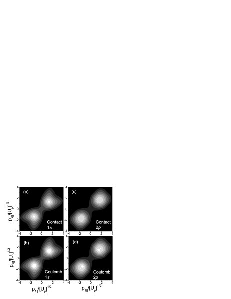
Figure 11: Electron momentum distributions computed with the modified form factors (35),(36), as functions of the electron momentum components parallel to the laser-field polarization, for same field and atomic parameters as in the previous figures. We consider that the ionic potential is of contact type (Eq. (34)), and use the saddle-point model without modifications (c.f. Sec. II). In the upper and lower panels, the electron-electron interaction $V_{12}$ was assumed to be of contact and Coulomb type, respectively. In panels (a), (b), both electrons are taken to be initially in $1s$ states, whereas in panels (c) and (d), they are initially in $2p$ states. The transverse momenta have been integrated over.

VI Conclusions

In this article, we have introduced several technical modifications in an S-Matrix theory of laser-induced nonsequential double ionization (NSDI), within the Strong-Field Approximation, in which this phenomenon is modeled as the inelastic collision of an electron with its parent ion. Such modifications include different initial bound states for the first and second electron, an adequate treatment of the bound-state singularity which exists in our framework, and an effective form factor which incorporates the residual ion. We performed a systematic analysis of their influence on the differential electron momentum distributions as functions of the parallel-momentum components $p_{j||}$, $(j=1,2)$ of both electrons.

Specifically, we consider that the second electron is dislodged by a contact- and Coulomb-type interaction, and assume that both electrons are initially in a $1s$, $2p$ or $3p$ hydrogenic state. As an additional case, we assume that the first electron is initially bound in a $1s$ state, and that the initial wave function of the second electron is localized at $\mathbf{r}_{2}=0.$ For the first electron, we take into account only the hydrogenic states, since a neutral atom, in contrast to a singly ionized atom, has a long-range binding potential.

Concerning the initial bound-state wave function of the second electron, our results show that the NSDI momentum distributions are very sensitive to its spatial extension, but not to its shape. Indeed, a spatially extended wave function causes a broadening in the electron momentum distributions along the anti-diagonal $p_{1||}=-p_{2||},$ even if the second electron is dislodged by a contact-type interaction. Circular-shaped distributions, as reported in pransdi1 ; pransdi2 and observed in experiments nsdireview ; expe1 are only obtained for a contact-type interaction under the additional condition that the bound-state wave function is localized at the origin of the coordinate system, i.e., at $\mathbf{r}_{2}=0.$ In addition to this broadening, if the second electron is released by a Coulomb-type interaction, there is an enhancement in the contributions near the axis $p_{1||}=0$ or $p_{2||}=0.$

All the distributions investigated in this article, however, change in a less radical fashion if the second electron is taken to be in a a $1s$, $2p$ or $3p$ hydrogenic state, as long as they exhibit a spatial extension. In fact, although specific changes are observed, such as an additional substructure for a Coulomb-type interaction, or more localized distributions for a contact-type interaction, the overall shapes of such distributions remains similar.

Furthermore, if the form factor $V_{\mathbf{k},0},$ which, within our model, contains all the influence of the initial state of the first electron, is incorporated in the time-dependent action, the only noticeable effect is a suppression in the yield, for regions of  small parallel momenta. Indeed, the distributions retain their shapes even if the saddle-point equations are modified in this way. Such changes have been introduced in order to correct a singularity which exists for such the prefactor $V_{\mathbf{k},0}$, within the saddle-point framework, if the initial bound state is exponentially decaying.

Finally, the inclusion of the ionic potential at the time of rescattering, as the modified form factors $\widetilde{V}_{\mathbf{p}_{j},\mathbf{k}}$, sheds some light on why, in the absence of the ion, a contact-type interaction localized at the origin of the coordinate system yields the best agreement with the experimental findings.

In fact, the ionic interaction leads to form factors which are very large near $p_{1||}=p_{2||}=\pm\sqrt{U_{p}}$. This causes an enhancement in the distributions in this region. If the ionic potential is of Coulomb type, this effect is overshadowed by the fact that $\eta(\mathbf{p}_{j},\mathbf{k})$, given by Eq. (22), favors unequal momenta. By contrast, if the ionic potential is given by Eq. (34), which is a good approximation for a short-range interaction, $\eta(\mathbf{p}_{j},\mathbf{k})=const.$ and the enhancement at the diagonal prevails. On the other hand, in Sec. III and IV, if $V_{\mathbf{p}_{j},\mathbf{k}}=const.$ (i.e., for $V_{12}$ of contact-type and a localized state for the second electron), the very same effect is caused by integrating over the phase space. Interestingly, if, in the presence of the ion, we consider $2p$ states, which are more realistic assumptions for our model, the agreement with the experimental findings improves even more.

In conclusion, the present results indicate that the ionic potential is an important ingredient for a realistic modeling of NSDI. Indeed, of all the technical modifications considered in this paper, which aimed at making the model more realistic, this was the only which played a major role in improving the agreement between theory and experiment. The other modifications either worsened this agreement, or had almost no influence on the momentum distributions. This supports the hypotheses raised in previous studies pransdi1 ; pransdi2 , that the residual ion might be screening both the long-range of the Coulomb interaction, or the final-state Coulomb repulsion, so that, effectively, the electron-electron interaction is of contact-type, and the bound-state wave functions are localized.

We would like to stress out, however, that the treatment performed in Sec. V is only a first approximation for a rigorous study of the ionic potential. There exist, in principle, more rigorous methods for incorporating the residual ion. The first approach would be to consider the ion as a further interaction in our model, and modify the transition amplitude accordingly. This is, however, a highly non-trivial task, since it would lead to one more rescattering and a further integral in the transition amplitude. Another possibility would be to incorporate the ionic potential in the propagation of both electrons in the continuum. This would allow a clear assessment of the Coulomb focusing, which, again, owes its existence to the presence of the ion. Indeed, this effect may as well be compensating the broadening caused by initial spatially extended wave functions. Definite statements on this issue, however, require a theoretical approach beyond the Strong-Field Approximation.

- (1) See, e.g., R. Dörner, T. Weber, W. Weckenbrock, A. Staudte, M. Hattass, H. Schmidt-Böcking, R. Moshammer, and J. Ullrich, Adv. At. Mol. Opt. Phys. 48, 1 (2002); J. Ullrich, R. Moshammer, A. Dorn, R. Dörner, L. Ph. H. Schmidt, H. Schmidt-Böcking, Rep. Prog. Phys. 66, 1463 (2003) for reviews on the subject.
- (2) R. Moshammer, B. Feuerstein, W. Schmitt, A. Dorn, C.D. Schröter, J. Ullrich, H. Rottke, C. Trump, M. Wittman, G. Korn, K. Hoffmann, and W. Sandner, Phys. Rev. Lett. 84, 447 (2000); Th. Weber, M. Weckenbrock, A. Staudte, L. Spielberger, O. Jagutzki, V. Mergel, F. Afaneh, G. Urbasch, M. Vollmer, H. Giessen, and R. Dörner, ibid. 84, 443 (2000).
- (3) B. Feuerstein, R. Moshammer, D. Fischer, A. Dorn, C.D. Schröter, J. Deipenwisch, J.R. Crespo Lopez-Urrutia, C. Höhr, P. Neumayer, J. Ullrich, H. Rottke, C. Trump, M. Wittmann, G. Korn and W. Sandner, Phys. Rev. Lett. 87, 043003 (2001); Th. Weber, H. Giessen, M. Weckenbrock, G. Urbasch, A. Staudte, L. Spielberger, O. Jagutzki, V. Mergel, M. Vollmer, R. Dörner, Nature 405, 658 (2000).
- (4) P. B. Corkum, Phys. Rev. Lett. 71, 1994 (1993); K. C. Kulander, K. J. Schafer, and J. L. Krause in: B. Piraux et al. eds., Proceedings of the SILAP conference, (Plenum, New York, 1993).
- (5) B. Feuerstein, R. Moshammer and J. Ullrich, J. Phys. B 33, L823 (2000); J. Chen, J. Liu, L.- B. Fu, and W. M. Zheng, Phys. Rev. A 63, 011404 (R)(2000); L. -B. Fu, J. Liu, J. Chen, and S. -G. Chen, ibid., 043416 (2001); J. Chen, J. Liu, and S. -G. Chen, Phys. Rev. A 65, 021406 (R)(2002); J. Chen, J. Liu, and W. M. Zheng, ibid. 66, 043410 (2002).
- (6) S. L. Haan, P. S. Wheeler, R. Panfili, and J. H. Eberly, Phys. Rev. A 66, 061402(R) (2002); R. Panfili, S. L. Haan and J. H. Eberly, Phys. Rev. Lett. 89, 113001 (2002).
- (7) X. Liu and C. Figueira de Morisson Faria, Phys. Rev. Lett. 92, 133006 (2004).
- (8) A. Becker and F.H.M. Faisal. Phys. Rev. A 50, 3256 (1994)
- (9) A. Becker and F.H.M. Faisal, Phys. Rev. Lett. 89, 193003 (2002); A. Jaron and A. Becker, Phys. Rev. A 67, 035401 (2003).
- (10) R. Kopold, W. Becker, H. Rottke and W. Sandner, Phys. Rev. Lett. 85, 3781 (2000); S. P. Goreslavskii, S. V. Popruzhenko, R. Kopold and W. Becker, Phys. Rev. A 64, 053402 (2002); S. V. Popruzhenko, Ph. A. Korneev, S. P. Goreslavskii, and W. Becker, Phys. Rev. Lett. 89, 023001 (2002); A. Heinrich, M. Lewenstein and A. Sanpera, J. Phys. B 37, 2087 (2004).
- (11) C. Figueira de Morisson Faria and W. Becker, Laser Phys. 13, 1196 (2003).
- (12) C. Figueira de Morisson Faria, X. Liu, W. Becker and H. Schomerus, Phys. Rev. A 69, 021402(R) (2004).
- (13) C. Figueira de Morisson Faria, H. Schomerus, X. Liu, and W. Becker, Phys. Rev. A 69, 043405 (2004).
- (14) C. Figueira de Morisson Faria, X. Liu, A. Sanpera and M. Lewenstein, Phys. Rev. A 70, 043406 (2004).
- (15) L.V. Keldysh, Zh. Éksp. Teor. Fiz. 47, 1945 (1964)[Sov. Phys. JETP 20, 1307 (1965)]; F. H. M. Faisal, J. Phys. B 6, L312 (1973); H. R. Reiss, Phys. Rev. A 22, 1786 (1980).
- (16) J.B. Watson, A. Sanpera, D. G. Lappas, P. L. Knight and K. Burnett, Phys. Rev. Lett. 78, 1884 (1997); D. Dundas, K. T. Taylor, J. S. Parker, and E. S. Smyth, J. Phys. B 32, L231 (1999); W. C. Liu, J. H. Eberly, S. L. Haan, R. Grobe, Phys. Rev. Lett. 83, 520 (1999); C. Szymanowski, R. Panfili, W. C. Liu, S. L. Haan, and J. H. Eberly, Phys. Rev. A 61, 055401 (2000); M. Lein, E. K. U. Gross, and V. Engel, Phys. Rev. Lett. 85, 4707 (2000).
- (17) See, e.g., P. Salières, B. Carré, L. Le Deroff, F. Grasbon, G. G. Paulus, H. Walther, R. Kopold, W. Becker, D. B. Milošević, A. Sanpera and M. Lewenstein, Science 292, 902 (2001); W. Becker, F. Grasbon, R. Kopold, D.B. Milošević, G.G. Paulus, and H. Walther, Adv. At. Mol. Opt. Phys.48, 35 (2002) and references therein.
- (18) G. L. Yudin, and M. Yu. Ivanov, Phys. Rev. A 63, 033404 (2001).
- (19) C. Figueira de Morisson Faria, H. Schomerus and W. Becker, Phys. Rev. A 66, 043413 (2002).
- (20) D. B. Milošević, and W. Becker, Phys. Rev. A 66, 063417 (2004); G. Sansone, C. Vozzi, S. Stagira and M. Nisoli, Phys. Rev. A 70, 013411 (2004); L.E. Chipperfield, L.N. Gaier, P.L. Knight, J.P. Marangos, and J.W.G. Tisch, J. Mod. Opt. 52, 243 (2005).
- (21) N. Bleistein and R. A. Handelsman, Asymptotic Expansions of Integrals (Dover, New York, 1986); H. Schomerus and M. Sieber, J. Phys. A 30, 4537(1997).
- (22) This effect can be described employing the Hartree-Fock approximation to compute bound states of neon, or argon. For a discussion of this method, see, e.g., H. Bethe and E.E. Salpeter, Quantum Mechanics of One and Two electron Atoms, (Plenum, New York, 1997); for applications of HF potentials for time dependent problems see K.C. Kulander, Phys. Rev . A 36, 2726 (1987); ibid. 38, 777 (1988); M.S. Pindzola, D.C. Griffin, and C. Bottcher, Phys. Rev. Lett. 66, 2305 (1991).