A Robust Estimation of the Exponent Function in the Gompertz Law

Abstract

The estimation of the solution of a system of two differential equations introduced by Norton et al. (1976) that is equivalent to the famous Gompertz growth law is performed by means of the recent adaptive scheme of Besançon and collaborators (2004). Results of computer simulations illustrate the robustness of the approach.

,  ,         &

1 Gompertz growth functions

Mathematically speaking, the Gompertz law refers to the class of functions having exponentially decreasing logarithmic derivatives. It has been introduced in 1825 by B. Gompertz in a paper on the law of human mortality Gomp1825 . He noted that for people between 40 and 100 years “the rate of mortality variable with age measures a force of death which grows each year by a fraction, always the same, of its present value”. According to Winsor Win , the possible application of the Gompertz curve in biology was first spelled out in 1926 by Sewall Wright in a few remarkable statements: “ In organisms, on the other hand, the damping off of growth depends more on internal changes in the cells themselves … The average growth power as measured by the percentage rate of increase tends to fall at a more or less uniform percentage rate, leading to asymmetrical types of s-shaped curves…”.

If the size $z(t)$ of a growing structure evolves according to the equation js03

$$\dot{z}=z\ln\left(\frac{S}{z}\right)~{},$$ (1)

we say that its growth is of Gompertz type. The evolution is continuous from a given initial stage to a plateau value $S$. In a Nature letter on the growth of tumours, Norton et al nor wrote the Gompertz law as the system of the following two first order differential equations

$$\dot{Z}_{1} = K_{1}Z_{1}Z_{2}$$ (2)

$$\dot{Z}_{2} = -K_{2}Z_{2}~{},$$ (3)

where $Z=(Z_{1},Z_{2})\in\mathbb{R}^{2}$, $K_{i}>0$, $Z_{1}$ is the volume of the tumour at time $t$, and $Z_{2}$ is a function entirely described by the second equation (3) that gives the difference in growth with respect to a pure exponential law. According to Norton, $K_{2}Z_{2}$ gives the fraction of the volume that doubles in size during the instant $dt$. Thus, $Z_{2}$ that we call for obvious reasons the Gompertzian exponent function is of special interest and we would like to determine it with high accuracy even though we know neither the initial conditions for $Z_{1}$ and $Z_{2}$ nor $K_{2}$. Norton et al wrote the solution of the system in the following form

$${Z}_{1}(t) = {Z}_{1}(0)\exp\left[\left(\frac{K_{1}}{K_{2}}\right){Z}_{2}(0)\left\{1-\exp(-K_{2}t)\right\}\right]~{},$$ (4)

$${Z}_{2}(t) = \left(\frac{K_{2}}{K_{1}}\right)\ln\left[\frac{S}{{Z}_{1}(t)}\right]~{}.$$ (5)

We will treat $Z_{1}$ and $Z_{2}$ as states of a dynamical system that in our case is the evolution of a tumour. The fundamental concept of state of a system or process could have many different empirical meanings in biology and in our case the first state $Z_{1}$ is just the size of the tumor whereas $Z_{2}$ is the deviation of the growth rate from the pure exponential growth. In general terms, a potentially useful tool in biology is the reconstruction of some specific states under conditions of limited information. For animal tumors, it is not trivial to know their state $Z_{1}$ at the initial moment and most often we do not know the instant of nucleation that can be determined only by extrapolation of the fitting to the analytic solutions of growth models, such as Eqs. (4) and (5). In this paper, the main goal is to show that an excellent alternative procedure for estimating the phenomenological quantities of the tumor growing process in the frequent case in which we do not know the initial conditions and the parameter $K_{2}$ is the recent adaptive scheme for state estimation proposed by Besançon and collaborators Besancon 2004 . In addition, what is generally measured, i.e., the output $y$, is a function of states that we denote by $h(Z)$ and in the particular case of tumors one usually measures their volume. Then:

$$y=h(Z)=Z_{1}~{}.$$ (6)

The mathematical formalism of the adaptive scheme that follows relies entirely on the Lie derivatives of the function $h(Z)$ that are defined in the next section. By a Lie mapping, we are able to write the Gompertz-Norton system in Besançon’s matrix form (system $\digamma$ below) that allows to write the corresponding adaptive algorithm (the dynamical system $\hat{\digamma}$ and its explicit Gompertz form $\hat{\digamma}_{G}$ below).

2 The adaptive scheme

Taking into account the fact that rarely one can have a sensor on every state variable, and some form of reconstruction from the available measured output data is needed, an algorithm can be constructed using the mathematical model of the process to obtain an estimate, say $\hat{X}$ of the true state $X$. This estimate can then be used as a substitute for the unknown state $X$. Ever since the original work by Luenberger Luenberger 1966 , the use of state ‘observers’ has proven useful in process monitoring and for many other tasks. The engineering concept of observer means an algorithm capable of giving a reasonable estimation of the unmeasured variables of a process using only the measurable output. Even more useful are the so-called adaptive schemes that mean observers that are able to provide an estimate of the state despite uncertainties in the parameters. The so-called high gain techniques proved to be very efficient for state estimation, leading in control theory to the well-known concept of high gain observer J.P.Gauthier92 . The gain is the amount of increase in error in the observer’s structure. This amount is directly related to the velocity with which the observer recovers the unknown signal. The high-gain observer is an algorithm in which the amount of increase in error is constant and usually of high values in order to achieve a fast recover of the unmeasurable states. In case of dynamical systems depending on unknown parameters, the design of the observer has to be modified appropriately in order that the state variables and parameters could be estimated. This leads to the so called adaptive observers, i.e., observers that can change in order to work better or provide more fit for a particular purpose. Recently, observers that do not depend on the initial conditions or the estimated parameters from the standpoint of asymptotic exponentially fast convergence to zero of the errors have been built for many systems. They are called globally convergent adaptive observers and have been obtained from a non trivial combination of a nonlinear high gain observer and a linear adaptive observer, see Zhang 2002 and Besancon 2004 . In this work, we present an application of the high gain techniques in the context of state estimation whatever the unknown parameter is.

The assumption on the considered class of systems are basically that if all of the parameters were known, some high-gain observer could be designed in a classical way, and that the system are “sufficiently excited” in a sense which is close to the usually required assumption on adaptive systems, that is, signals should be dynamically rich enough so that the unknown parameters can indeed be identified. In this particular case, the lack of persistent excitation of the system could impede the reconstruction of the parameters. However, the recent scheme of Besançon and collaborators Besancon 2004 guarantees the accurate estimation of the states according to rigorous arguments in their paper.

To make this mathematically precise we have to introduce first some terminology. Let us construct the $j$th time derivative of the output. This can be expressed using Lie differentiation of the function $h$ by means of the vector field $f$ given by the right hand sides of Norton’s system. We will denote the $j$th Lie derivative of $h$ with respect to $f$ by ${L_{f}}^{j}\left(h\right)\left(Z(t)\right)$. These Lie derivatives are defined inductively as functions of $Z$

$${L_{f}}^{0}\left(h\right)\left(Z\right) = h\left(Z\right)$$

$${L_{f}}^{j}\left(h\right)\left(Z\right) = \frac{\partial}{\partial Z}\left({L_{f}}^{j-1}\left(h\right)\left(Z\right)\right)f(Z)~{}.$$

When the system is observable, i.e., from the knowledge of the output one can build the states of the system, the Lie map $\Phi:Z\rightarrow\Phi(Z)$ given by

$$\xi=\Phi(Z)=\left(\begin{array}[]{c}h(Z)\\ {L_{f}}\left(h(Z)\right)\end{array}\right)=\left[\begin{array}[]{c}Z_{{1}}\\ K_{{1}}Z_{{1}}Z_{{2}}\end{array}\right]$$ (11)

is a diffeomorphism. For $\Phi(Z)$ to be a diffeomorphism on a region $\Omega$, it is necessary and sufficient that the Jacobian $\mathrm{d}\Phi(Z)$ be nonsingular on $\Omega$ and that $\Phi(Z)$ be one-to-one from $\Omega$ to $\Phi(\Omega)$, see Shim .

Since $\Phi(Z)$ is a diffeomorphism, one can write the global coordinate system defined by $X=\Phi(Z)$ in the following form

$$\Upsilon:\ \ \ \left\{\begin{array}[]{c}\dot{X}_{1}=X_{2}\\ \dot{X}_{2}=\frac{{X_{2}}^{2}}{X_{1}}-K_{2}X_{2}\\ y=X_{1}\end{array}\right.~{}.$$ (15)

Following Besancon 2004 , we assume that the $\Upsilon$ system can be written in the matrix form as follows

$$\left.\begin{array}[]{@{}l@{\quad}l@{}}\dot{X}=AX+\varphi(X)+\Psi(X)\theta\\ y=CX\end{array}\ \right\}\,\equiv\digamma\,,$$

where $X\in\mathbb{R}^{n}$, $A=\left[\begin{array}[]{cc}0&1\\ 0&0\end{array}\right]$, $\varphi(X)=(0,\frac{X_{2}^{2}}{X_{1}})^{T}$, $y$ is the measured output, $\Psi(t)\in\mathbb{R}^{n\times p}$ is the matrix of known functions and $\theta\in\mathbb{R}^{p}$ is the vector of unknown parameters that should be estimated through the measurements of the output $y$. We are here in the particular case $n=2,\,p=1$, i.e., $\Psi(t)=[0,-X_{2}]^{T}$ and $\theta\in\mathbb{R}^{1}=K_{2}$. In addition, the algorithm we develop is a particular case of that presented in Besancon 2004 , since we can not meddle in the system, in other words, there is no control input. As adaptive observer we use the system Besancon 2004

$$\hat{\digamma}\equiv\left\{\begin{array}[]{l}\dot{\hat{X}}=A\hat{X}+\varphi(\sigma(\hat{X}))+\Psi(\sigma({\hat{X}}))\sigma({\theta})+\Lambda^{-1}\left[\rho\mathcal{K}+\Gamma\Gamma^{T}C^{T}\right]\left(y-C\hat{X}\right)\\ \dot{\hat{\theta}}=\left[\rho^{n}\Gamma^{T}C^{T}\right]\left(y-C\hat{X}\right)\\ \dot{\Gamma}=\rho\left(A-\mathcal{K}C\right)\Gamma+\rho\Psi(\sigma(\hat{X}))\end{array}\right.$$ (16)

where $\sigma(\cdot)$ is a saturation function, $\Gamma\in\mathbb{R}^{n\times p}$ is the so-called gain vector, $\mathcal{K}$ is a vector that makes $A-\mathcal{K}C$ a stable matrix, $\Lambda={\rm diag}[1,\rho^{-1},\ldots,\rho^{-(n-1)}]$ where $\rho\in\mathbb{R}_{+}$ is a constant to be chosen. The saturation function is a map whose image is bounded by chosen upper and lower limits, $B$ and $b$, respectively. It is customary to introduce such functions of simple forms, e.g., we used

$$\sigma(s)=\\ \ \left\{\begin{array}[]{l}B$\quad\quad$s>B\\ s$\quad\quad$b\leq s\leq B\\ b$\quad\quad$s<b~{},\end{array}\right.$$

to avoid the over and/or underestimation and in this way to increase the chance of the quick convergence to the true value Khalil .

In Besancon 2004 , it is proven that the dynamical system $\hat{\digamma}$ is a global exponential adaptive observer for the system $\digamma$, i.e., for any initial conditions $X(t_{0})$, $\hat{X}(t_{0})$, $\hat{\theta}(t_{0})$ and $\forall\theta\in\mathbb{R}^{p}$, the errors $\hat{X}(t)-X(t)$ and $\hat{\theta}(t)-\theta(t)$ tend to zero exponentially fast when $t\rightarrow\infty$. Taking $\mathcal{K}=[\mathcal{K}_{1},\mathcal{K}_{2}]$, the matrix $A-\mathcal{K}C$ have the following eigenvalues

$$\lambda_{1,2}=-1/2\,\mathcal{K}_{{1}}\pm 1/2\,\sqrt{{\mathcal{K}_{{1}}}^{2}-4\,\mathcal{K}_{{2}}}~{}.$$ (17)

Selecting $\mathcal{K}_{{2}}=(1/4)\,{\mathcal{K}_{{1}}}^{2}$, we get equal eigenvalues $\lambda_{1}=\lambda_{2}=-(1/2)\,\mathcal{K}_{{1}}$, and choosing $\mathcal{K}_{1}>0$ we turn $A-\mathcal{K}C$ into a stable matrix. Thus, the explicit form of the observer system $\hat{\digamma}$ is given by

$$\hat{\digamma}_{G}=\\ \ \left\{\begin{array}[]{l}\dot{\hat{X}}_{1}=\hat{X}_{2}+\left(\rho\mathcal{K}_{1}+{\Gamma_{1}}^{2}\right)(X_{1}-\hat{X}_{1})\\ \dot{\hat{X}}_{2}=\frac{\left(\sigma(\hat{X}_{2})\right)^{2}}{\sigma(\hat{X}_{1})}-\sigma(\hat{X}_{2})\sigma(\hat{\theta})+\rho\left(\frac{\rho{\mathcal{K}_{1}}^{2}}{4}+\Gamma_{1}\Gamma_{2}\right)(X_{1}-\hat{X}_{1})\\ \dot{\hat{\theta}}=\rho^{2}\Gamma_{1}(X_{1}-\hat{X}_{1})\\ \dot{\Gamma}_{1}=\rho(-\mathcal{K}_{1}\Gamma_{1}+\Gamma_{2})\\ \dot{\Gamma}_{2}=-\frac{\rho{\mathcal{K}_{1}}^{2}\Gamma_{1}}{4}+\rho\sigma(\hat{X}_{2})~{}.\end{array}\right.$$

Being global, this observer system does not depend on the initial conditions. Therefore, any initial conditions chosen at random from a set of physical values will not affect the correct estimation; merely the convergence time could be longer or shorter. Thus, in practice, it is useful to start with initial conditions that are close to the real phenomenological initial conditions in a given framework.

Finally, to recover the original states, we use the inverse transformation $\Phi^{-1}(\hat{X})$, which is given by:

$$\hat{Z}=\xi^{-1}=\Phi^{-1}(\hat{X})=\left(\begin{array}[]{c}\hat{Z}_{1}\\ \hat{Z}_{2}\end{array}\right)=\left(\begin{array}[]{c}\hat{X}_{{1}}\\ \frac{\hat{X}_{{2}}^{2}}{K_{{1}}\hat{X}_{{1}}}\end{array}\right)~{}.$$ (22)

With the aim of better illustrating the adaptive scheme proposed here, we present numerical simulations. We use the following values of the parameters: $K_{1}=1$, $K_{2}=0.5$, $\rho=100$ and $\mathcal{K}_{1}=1$. In Figs. (1) and (2), the solid lines represent the evolution of the true states and the dotted lines stand for the evolution of the estimates, respectively. We mention that short convergence time is what really matters in order to have efficient numerical simulations. This can be accomplished by starting with arbitrary initial conditions that are guessed to be close to the real initial ones as we already commented. If one is interested in the evolution of the iterative scheme, this can be readily glimpsed from the difference $\hat{Z}_{i}-Z_{i}$ between the curves in the figures.

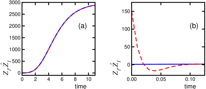
Figure 1: Numerical simulation for the first state: (a) the solid line represents the time evolution of the true states $Z_{1}$ and the dotted line represents the estimate $\hat{Z}_{1}$. Plot (b) is a detail of (a) to appreciate the variation of $\hat{Z}_{1}$ in the beginning.

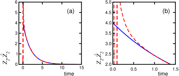
Figure 2: Numerical simulation for the second state: (a) the solid line represents the true state $Z_{2}$ and the dotted line represents the estimate $\hat{Z}_{2}$. Plot (b) is a detail of (a) in order to appreciate better the variation of $\hat{Z}_{2}$ in the beginning.

To this end, we would like to illustrate the robustness of the present adaptive scheme. Figs. (3) and (4) show what happens when an impulsive type perturbation (i.e., of high value acting in a very short span of time) is added to the output signal $h(Z)=Z_{1}$ which is fed to the observer at $t=4$ (arbitrary units). This perturbation is a strong error in the output $y$ that can be attributed to an unexpected fault in a measurement device or even human errors and does not belong to the natural evolution of the tumour. As can be seen from the graphics, the adaptive scheme has the ability to recover the “true” signal immediately after the perturbation disappears. In general, this robustness is due to the fact that the scheme is designed in the closed-loop way and additionally not the full range of the parameters need to be known.

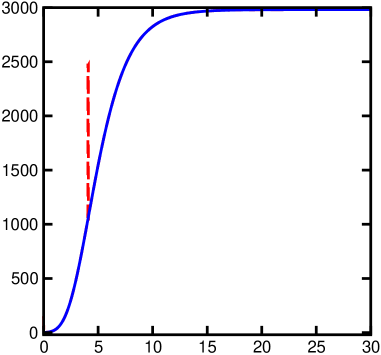
Figure 3: Behaviour of $Z_{1}$, $\hat{Z}_{1}$ under an impulse-type perturbation at $t=4$ (arbitrary units).

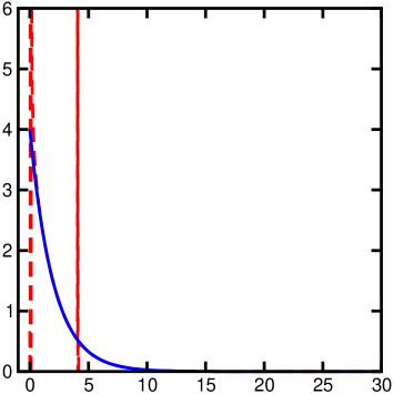
Figure 4: Behaviour of $Z_{2}$, $\hat{Z}_{2}$ under the same perturbation at $t=4$ (arbitrary units).

3 Conclusion

The robust adaptive scheme we used here for the interesting case of Gompertz growth functions is a version of that due to Besançon et al. The results of this work indicate that this scheme is very efficient in obtaining the Gompertz functions without knowing both initial conditions and parameter $K_{2}$. The method may be useful in more general frameworks for models of self-limited growth such as in the construction of a specific growth curve in biology, or as a managerial tool in livestock enterprizes, as well as in the detailed understanding of the growth of tumors. We also notice that the reconstruction of the unknown states by this method allows the possibility to obtain important missing parameters by standard fitting procedures.

References

- (1) Gompertz B., On the nature of the function expressive of the law of human mortality, Phil. Trans. Roy. Soc. A 115 (1825) pp. 513-585.
- (2) Winsor C.P., The Gompertz curve as a growth curve, Proc. Nat. Acad. Sci. 18 (1932) pp. 1-8.
- (3) D.S. Jones and B.D. Sleeman, Differential Equations and Mathematical Biology, (Chapman & Hall CRC Press Company, 2003) p. 18.
- (4) Norton L., Simon R., Brereton H.D., Bogden A.E., Predicting the course of Gompertzian growth, Nature 264 (1976) pp. 542-544.
- (5) Besançon G., Zhang Q., Hammouri H., High gain observer based state and parameter estimation in nonlinear systems, paper 204 The 6th IFAC symposium, Stuttgart Symposium on Nonlinear Control Systems (NOLCOS) (2004), available at http://www.nolcos2004.uni-stuttgart.de
- (6) D. Luenberger, Observers for multivariable systems, IEEE Trans. Autom. Control 11, 190 (1966).
- (7) J.P. Gauthier, H. Hammouri, and S. Othaman, A simple observer for nonliner systems applications to bioreactors, IEEE Trans. Aut. Ctrl. 37, 875 (1992).
- (8) Zhang Q., Adaptive observer for multiple-input multiple-output (MIMO) linear time varying systems, IEEE Trans. Aut. Ctrl. 47 (2002) pp. 525-529.
- (9) Shim H., Son Y.I., and Seo J.H., Semi-global observer for multi-output nonlinear systems, Systems & Control Letters 41 (2001) pp. 233-244.
- (10) H.K. Khalil, Nonlinear Systems, (Prentice-Hall, Inc., 1992).