Spectral Properties and Lifetimes of Neutral Spin-$\frac{1}{2}$-Fermions in a Magnetic Guide

Abstract

We investigate the resonant motion of neutral spin-$\frac{1}{2}$-fermions in a magnetic guide. A wealth of unitary and anti-unitary symmetries is revealed in particular giving rise to a two-fold degeneracy of the energy levels. To compute the energies and decay widths of a large number of resonances the complex scaling method is employed. We discuss the dependence of the lifetimes on the angular momentum of the resonance states. In this context the existence of so-called quasi-bound states is shown. In order to approximately calculate the resonance energies of such states a radial Schrödinger equation is derived which improves the well-known adiabatic approximation. The effects of an additionally applied homogeneous Ioffe field on the resonance energies and decay widths are also considered. The results are applied to the case of the ${}^{6}\text{Li}$ atom in the $F=\frac{1}{2}$ hyperfine ground state.

I Introduction

Magnetic traps are now being used for many years in order to study and manipulate the properties of neutral atoms Folman02 . With the availability of efficient cooling techniques the controlled occupation of low lying quantum levels inside such traps became possible. This paved the way for the experimental exploration of several phenomena such as Bose-Einstein-condensation (see Ref. Pethick02 and references therein) or the formation of degenerate Fermi gases Schreck01 . Apart from studying such collective properties there is also a fundamental and vivid interest in the properties and the dynamics of single atoms. Its understanding is essential in order to identify systems for quantum information processing but it is also necessary to gain insights into trapping mechanisms in order to control the atomic motion. Theoretical studies of the quantum properties of neutral atoms in magnetic traps have been performed since the late eighties. Since then several field configurations have been in the focus of numerous publications, e.g. the quadrupole field Bergeman89 , the wire trap Hau95 ; Berg-Soerensen96 ; Burke96 or the magnetic guide and the Ioffe trap Hinds00 ; Hinds00E ; Potvliege01 . However, only a few field configurations allow for stationary solutions. Bound states of spin-$\frac{1}{2}$-particles trapped by a wire have been found analytically by Blümel et al. Bluemell91 and Vestergaard Hau et al. Hau95 . The latter authors employed a super-symmetric approach in order to derive the Rydberg series of bound states around an infinitely thin wire. Finite wire sizes were accounted for by introducing a quantum defect in the Rydberg formula. Burke et al. Burke96 were able to numerically derive similar series of energies for particles with spin up to 2 by using the finite element method combined with the application of multichannel quantum defect theory. However, in most cases atoms are trapped in meta-stable states which have a finite lifetime. The calculation of the corresponding resonance energies and lifetimes requires the application of sophisticated numerical methods. Bergeman et al. Bergeman89 have calculated dozens of resonances of spin-$\frac{1}{2}$-particles inside a three-dimensional magnetic quadrupole field by determining the phase-shift of scattered waves. A similar approach was pursued by Hinds and Eberlein Hinds00 ; Hinds00E which have studied the dynamics of neutral particles in a magnetic guide. Their results were reproduced by Potvliege and Zehnlé who have performed a complex scaling calculation. In both publications the effect of an additionally applied homogeneous Ioffe field is also discussed but only a few resonances are studied. Although there are no principle obstacles to compute resonances there has always been put great effort in finding reasonable approximations which allow for an quick and easy calculation of the resonance energies. Here the most prominent example is the so-called adiabatic approximation Bergeman89 ; Berg-Soerensen96 where the spin is aligned along the local direction of the magnetic field. Depending on their electronic state the atoms are here divided into low- and high-field seekers which give rise to bound and unbound solutions.

In this work we focus on the quantum dynamics of a neutral spin-$\frac{1}{2}$-particle in a magnetic guide. We also address the case of an additional homogeneous field being applied parallel to the guide (Ioffe field). Like Potvliege and ZehnléPotvliege01 we employ a complex scaling approach. In contrast to their work we calculate hundreds of resonances for several values of the Ioffe field strength which enables us to analyze global features of the resonance spectrum. In order get further insights we develop an approximate description of so-called quasi-bound states. We derive a radial Schrödinger equation which is superior to the common adiabatic approach. In contrast to the latter our method becomes exact for high angular momenta and its quality does not depend on whether there is an additional Ioffe field or not.

This work is organized as follows: In Section II we derive the Hamiltonian for a neutral particle possessing a magnetic moment $\vec{\mu}$ in a magnetic guide. We also account for an eventually applied homogeneous Ioffe field parallel to the guide. The resulting two-dimensional Hamiltonian depends on a single parameter involving both the gradient of the inhomogeneous field and the Ioffe field strength. It exhibits a plethora of unitary as well as anti-unitary symmetries. The effects of this intricate symmetry properties and in particular a resultant two-fold degeneracy of the resonance energies are discussed in Sec. III. In Sec. IV we briefly outline the numerical approach we pursue in order to obtain the resonance energies and decay width which is based on the complex scaling method. Sec. V is devoted to a discussion of our results. We analyze the resonance spectrum for several values of the Ioffe field strength. Furthermore we investigate how the energies and lifetimes of the resonance states depend on their angular momentum. The properties of so-called quasi bound states are addressed. We provide a radial Schrödinger equation whose eigenenergies are very good approximations of the true resonance energies. A comparison to the commonly used adiabatic approximation is also performed. Finally the results are applied to the case of ${}^{6}\text{Li}$ in a magnetic field generated by a current carrying wire together with a homogeneous bias field.

II The Hamiltonian

We consider the motion of a neutral spin-$\frac{1}{2}$-particle which carries the magnetic moment $\vec{\mu}$ inside a magnetic quadrupole guide. The magnetic field is given by

$$\vec{B}\left(\vec{r}\right)=\left(\begin{array}[]{c}b\,x\\ -b\,y\\ B\\ \end{array}\right).$$ (4)

The parameters $b$ and $B$ determine the gradient and the field strength of an eventually applied homogeneous field along the $z$-axis (Ioffe field), respectively. Generally the Hamiltonian for a neutral particle with the magnetic moment $\vec{\mu}$ and mass $M$ in a magnetic field reads

$$H_{3D}=\frac{1}{2M}\left(p_{x}^{2}+p_{y}^{2}+p_{z}^{2}\right)-\vec{\mu}\cdot\vec{B}\left(\vec{r}\right)$$ (5)

Since there is in our case (5) no explicit dependence on the $z$-coordinate the momentum in $z$-direction $p_{z}$ is conserved. Employing plane waves for the wavefunction in $z$-direction one obtains a two-dimensional Hamiltonian which describes the dynamics in the $x-y$ plane. Adopting atomic units and with $\vec{\mu}=-\frac{g}{2}\vec{S}$ where $\vec{S}$ is the spin operator one yields

$$H_{2D}=\frac{1}{2M}\left[p_{x}^{2}+p_{y}^{2}+\frac{gM}{2}\left(b\,x\sigma_{x}-b\,y\sigma_{y}+B\,\sigma_{z}\right)\right].$$ (6)

Here $g$ is the $g$-factor of the particle. The components of $\vec{S}$ are given through the Pauli matrices $\sigma_{i}$. Performing the scale transformation $\bar{x}_{i}=\left(\frac{bgM}{2}\right)^{\frac{1}{3}}x_{i}$ and $\bar{p}=\left(\frac{bgM}{2}\right)^{-\frac{1}{3}}p_{i}$ and omitting the bars one obtains

$$M\left(\frac{bgM}{2}\right)^{-\frac{2}{3}}H_{2D}=H=\frac{1}{2}\left(p_{x}^{2}+p_{y}^{2}+x\sigma_{x}-y\sigma_{y}+\gamma\,\sigma_{z}\right)$$ (7)

with $\gamma=B\left(\frac{gM}{2b^{2}}\right)^{\frac{1}{3}}$. For $\gamma=0$ the gradient $b$ does not explicitly appear in equation (7). Therefore we find here the energy level spacing to scale according to $\frac{1}{M}\left(\frac{bgM}{2}\right)^{\frac{2}{3}}$.

III Symmetries

III.1 The case $\gamma=0$

Analyzing the structure of the Hamiltonian (7) for $\gamma=0$ we find 15 discrete symmetry operations. They are listed in table 1.

$\Sigma_{x}=\sigma_{x}P_{y}$	$\Sigma_{y}=P_{x}\sigma_{y}$	$\Sigma_{z}=P_{x}P_{y}\sigma_{z}$
$I_{xy}S_{1}$	$P_{y}I_{xy}S_{2}$	$P_{x}P_{y}I_{xy}S_{1}^{*}$	$P_{x}I_{xy}S_{2}^{*}$
$T\sigma_{x}$	$TP_{x}P_{y}\sigma_{y}$	$TP_{x}\sigma_{z}$	$TP_{y}$
$TP_{y}I_{xy}S_{1}$	$TI_{xy}S_{2}$	$TP_{x}I_{xy}S_{1}^{*}$	$TP_{x}P_{y}I_{xy}S_{2}^{*}$

Table 1: Symmetry operations of the Hamiltonian (7) for $\gamma=0$. Top part: unitary symmetries. Bottom part: anti-unitary symmetries.

Each symmetry is composed of a number of elementary operations which are provided in table 2.

Operator	Operation
$P_{x_{i}}$	$x_{i}\rightarrow-x_{i}$
$T$	$A\rightarrow A^{*}$
$\sigma_{x}$	$\sigma_{y}\rightarrow-\sigma_{y}$ $\sigma_{z}\rightarrow-\sigma_{z}$
$\sigma_{y}$	$\sigma_{x}\rightarrow-\sigma_{x}$ $\sigma_{z}\rightarrow-\sigma_{z}$
$\sigma_{z}$	$\sigma_{x}\rightarrow-\sigma_{x}$ $\sigma_{y}\rightarrow-\sigma_{y}$
$I_{xy}$	$x\rightarrow y$ $y\rightarrow x$  ($\phi\rightarrow-\phi+\frac{\pi}{2}$)
$S_{1}=\left(\begin{array}[]{cc}0&1\\ -i&0\\ \end{array}\right)$	$\sigma_{x}\rightarrow-\sigma_{y}$ $\sigma_{y}\rightarrow-\sigma_{x}$ $\sigma_{z}\rightarrow-\sigma_{z}$
$S_{2}=\left(\begin{array}[]{cc}-i&0\\ 0&1\\ \end{array}\right)$	$\sigma_{x}\rightarrow-\sigma_{y}$ $\sigma_{y}\rightarrow\sigma_{x}$ $\sigma_{z}\rightarrow\sigma_{z}$

Table 2: Set of discrete operations out of which all symmetry operations of the Hamiltonian (7) can be composed.

All symmetry operations are either unitary or anti-unitary, the anti-unitary ones involving the conventional time reversal operator $T$. In spite of its simplicity the system (7) possesses a wealth of symmetry properties. The algebra of the underlying symmetry group possesses a complicated structure some features of which will be discussed in the following. The operators $\Sigma_{x}$, $\Sigma_{y}$ and $\Sigma_{z}$ generate a sub-group obeying the algebra $\left[\Sigma_{i},\Sigma_{j}\right]=2i\,\epsilon_{ijk}\Sigma_{k}$ reminiscent of angular momentum operators. In addition one finds $\Sigma_{i}^{2}=1$. Interestingly these quantities act on both real and spin space.

Apart from the discrete symmetries there is a continuous symmetry namely $\Lambda_{z}=L_{z}-S_{z}$ which was already pointed out by Eberlein and Hinds in Ref. Hinds00E . The operator $\Lambda_{z}$ obeys the eigenvalue equation

$$\Lambda_{z}\left|m\right>=m\left|m\right>$$ (8)

with the half-integer quantum numbers $m$. For spin-$\frac{1}{2}$-particles the states $\left|m\right>$ read in the spatial representation

$$\left|m\right>=\left(\begin{array}[]{c}\alpha^{\uparrow}\,e^{i(m+\frac{1}{2})\phi}\\ \alpha^{\downarrow}\,e^{i(m-\frac{1}{2})\phi}\\ \end{array}\right).$$ (11)

The symmetries listed in table 1 together with $\Lambda_{z}$ allow several sets of commuting operators. For our investigation we choose the set consisting of $H$, $\Sigma_{z}$ and $\Lambda_{z}$. Calculating the eigenvalue of a $\Lambda_{z}$ eigenstate with respect to the $\Sigma_{z}$ operator leads to

$$\Sigma_{z}\left|m\right>=\left(\begin{array}[]{c}\alpha^{\uparrow}\,e^{i(m+\frac{1}{2})(\phi+\pi)}\\ -\alpha^{\downarrow}\,e^{i(m-\frac{1}{2})(\phi+\pi)}\\ \end{array}\right)=e^{i(m+\frac{1}{2})\pi}\left|m\right>=\kappa\left|m\right>.$$ (14)

Therefore in case of $m+\frac{1}{2}$ being odd we find $\kappa=-1$ whereas we obtain $\kappa=1$ for even values of $m+\frac{1}{2}$.

Exploiting the discrete symmetries one can show that there is a two-fold degeneracy of any energy level. This degeneracy is revealed as follows. The operations $\Sigma_{z}$ and $P_{y}\sigma_{x}$ obey $\left\{\Sigma_{z},P_{y}\sigma_{x}\right\}=0$. Let $\left|E,\kappa\right>$ be an energy eigenstate and at the same time an eigenstate of $\Sigma_{z}$ with

$$\Sigma_{z}\left|E,\kappa\right> = \kappa\left|E,\kappa\right>$$ (15)

and $\kappa=\pm 1$. Employing the above anti-commutator one obtains

$$\Sigma_{z}P_{y}\sigma_{x}\left|E,\kappa\right>=-P_{y}\sigma_{x}\Sigma_{z}\left|E,\kappa\right>=-\kappa P_{y}\sigma_{x}\left|E,\kappa\right>$$ (16)

The state $P_{y}\sigma_{x}\left|E,\kappa\right>$ can be identified with $\left|E,-\kappa\right>$. Hence, as long as $\kappa\neq 0$ there is always an orthogonal pair of states possessing the same energy namely $\left|E,\kappa\right>$ and $\left|E,-\kappa\right>$. We have to emphasize that there occur no further degeneracies in the system. In principle one could think of performing the above calculation repeatedly but now substituting $P_{y}\sigma_{x}$ with any operator listed in table 1 which anti-commutes with $\Sigma_{z}$. It turns out that all of the resulting states generated by this scheme are either superpositions of $\left|E,\kappa\right>$ and $\left|E,-\kappa\right>$ or differ only by a phase factor from one of these states.

Since $\Sigma_{z}$ and $\Lambda_{z}$ commute, i.e. $\left[\Sigma_{z},\Lambda_{z}\right]=0$, one can construct eigenstates with respect to both of these operators: $\left|E,m,\kappa\right>$. Letting $P_{y}\sigma_{x}$ act on these states together with considering the anti-commutator $\left\{P_{y}\sigma_{x},\Lambda_{z}\right\}=0$ one finds

$$\Lambda_{z}\,P_{y}\sigma_{x}\left|E,m,\kappa\right>=-P_{y}\sigma_{x}\,\Lambda_{z}\left|E,m,\kappa\right>=-m\,P_{y}\sigma_{x}\left|E,m,\kappa\right>.$$ (17)

Hence we can identify $P_{y}\sigma_{x}\left|E,m,\kappa\right>$ with $\left|E,-m,\kappa\right>$. Therefore the pairs of degenerate states do not only have opposite $\kappa$ quantum number but also opposite $m$-values. A detailed discussion of degeneracies of spin-$\frac{1}{2}$-particles can be found in Lesanovsky04 .

III.2 The case $\gamma\neq 0$

For $\gamma\neq 0$ the conserved quantity $\Lambda_{z}$ persists but only 7 of the discrete symmetries for $\gamma=0$ remain. They are listed in table 3.

$\Sigma_{z}$	$P_{y}I_{xy}S_{2}$	$P_{x}I_{xy}S_{2}^{*}$
$TP_{y}$	$TP_{x}\sigma_{z}$	$TP_{x}P_{y}I_{xy}S_{2}^{*}$	$TI_{xy}S_{2}$

Table 3: Discrete symmetry operations of the Hamiltonian (7) for a finite Ioffe field strength $B$, i.e. $\gamma\neq 0$. Top part: unitary symmetries. Bottom part: anti-unitary symmetries. symmetries.

These operations form a non-Abelian algebra. In contrast to the group operations listed in table 1 there are no two anti-commuting operators. Hence it is not possible to construct pairs of degenerate energy eigenstates as discussed above. The operation $P_{y}\sigma_{x}$ which we have used to construct the degenerate pairs of states for $\gamma=0$ now has the following property

$$P_{y}\sigma_{x}\,H\left(\gamma\right)\,P_{y}\sigma_{x}=H\left(-\gamma\right),$$ (18)

i.e. the sign of $\gamma$ in the Hamiltonian (7) is changed. Hence, the application of $P_{y}\sigma_{x}$ reverses the sign of the homogeneous Ioffe field. We emphasize that even for $\gamma\neq 0$ the operators $H$, $\Sigma_{z}$ and $\Lambda_{z}$ form a commuting set of operators.

IV Numerical Treatment

The Hamiltonian (7) does not support bound states Hinds00E . In order to calculate the energies and decay widths of the scattering wavefunctions we employ the complex scaling method together with the linear variational principle.

We perform a rotation of the spatial coordinates into the complex plane: $x_{i}\rightarrow x_{i}e^{i\theta}$ which yields the ’rotated’ Hamiltonian

$$H\left(\theta\right)=\frac{1}{2}\left(p_{x}^{2}e^{-i2\theta}+p_{y}^{2}e^{-i2\theta}+xe^{i\theta}\sigma_{x}-ye^{i\theta}\sigma_{y}\right).$$ (19)

Unlike the bound states only continuum states are affected by the complex scaling procedure. The scattering states are rotated into the lower half of the complex plane and in particular resonances correspond now to square integrable functions. Since for $\theta\neq 0$ the complex scaled Hamiltonian (19) is not Hermitian one encounters complex energies:

$$\varepsilon=E-i\frac{\Gamma}{2}.$$ (20)

Here $E$ is the energy and $\Gamma$ the decay width of the resonance (the lifetime $\tau$ of a quantum states is connected to its decay width by $\tau=\Gamma^{-1}$). In general the energy $E$ will depend on the value of the rotation angle $\theta$. Continuum states are rotated by $2\theta$ into the lower half of the complex plane whereas energies of resonance states - once revealed - are independent of the angle $\theta$. A detailed discussion of the complex scaling procedure can be found in Ref. Moiseyev98 and Refs. therein. Since the complex scaling procedure transforms resonance states into square integrable wavefunctions one can apply the linear variational principle in order to compute the wavefunctions and resonance energies. We utilize an orthonormal basis set of the form

$$\left|m,n,s\right>=\left|m,n\right>\left|s\right>$$ (21)

where the functions $\left|n,m\right>$ are products of harmonic oscillator eigenfunctions

$$\left|m,n\right>=\frac{\sqrt[4]{\omega_{x}\omega_{y}}}{\sqrt{2^{m+n}\pi\,m!\,n!}}\,e^{-\frac{1}{2}\left(\omega_{x}x^{2}+\omega_{y}y^{2}\right)}H_{m}\left(\sqrt{\omega_{x}}x\right)H_{n}\left(\sqrt{\omega_{y}}y\right)$$ (22)

The parameters $\omega_{x}$ and $\omega_{y}$ are non-linear variational parameters which can be adapted in order to gain an optimal convergence behavior of the numerically obtained wavefunctions. To cover the spin space dynamics we utilize the spinor-orbitals $\left|s\right>=\left|\downarrow\right>$ and $\left|\uparrow\right>$, respectively. Performing the linear variational principle the solutions $\left|E\right>$ of the stationary Schrödinger equation are expanded in a finite set of the functions (22):

$$\left|E\right>=\sum_{nms}c_{mn}\left|m,n,s\right>$$ (23)

From our knowledge of the symmetry properties we can choose a more specific appearance of this expansion. Requiring the states $\left|E\right>$ to be eigenstates with respect to $\Sigma_{z}$ we make use of the properties

$$\Sigma_{z}\left|m,n,\uparrow\right> = \left(-1\right)^{m+n}\left|m,n,\uparrow\right>$$ (24)

$$\Sigma_{z}\left|m,n,\downarrow\right> = \left(-1\right)^{m+n+1}\left|m,n,\downarrow\right>.$$ (25)

Thus the expansions for the two $\kappa$ subspaces read

$$\left|E,\kappa=+1\right> = \sum_{m+n=\text{even}}a_{mn}\left|m,n,\uparrow\right>+\sum_{m+n=\text{odd}}b_{mn}\left|m,n,\downarrow\right>$$ (26)

$$\left|E,\kappa=-1\right> = \sum_{m+n=\text{odd}}a_{mn}\left|m,n,\uparrow\right>+\sum_{m+n=\text{even}}b_{mn}\left|m,n,\downarrow\right>.$$ (27)

Since $\left[\Lambda_{z},\Sigma_{z}\right]=0$ one could also demand the states to be a priori eigenfunctions of $\Lambda_{z}$ as well. However, our basis set is not particularly well suited to construct eigenfunctions to $\Lambda_{z}$. We therefore abstain from putting this constraint on the above expansion. Nevertheless, the resulting diagonalization of the Hamiltonian matrix (see below) guarantees that our numerically obtained energy and $\Sigma_{z}$-eigenfunctions are also eigenfunctions to $\Lambda_{z}$.

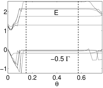
Figure 1: Dependence of the resonance energies (upper part) and decay widths (lower part) on the complex scaling angle $\theta$ as observed in the numerical calulations. The stationary region is located in between the dashed lines.

The determination of the optimal expansion coefficients $a_{mn}$ and $b_{mn}$ gives rise to a complex algebraic eigenvalue problem $\mathbf{H}\left(\theta\right)\vec{v}\left(\theta\right)=\varepsilon\left(\theta\right)\vec{v}\left(\theta\right)$, where $\mathbf{H}$ is the matrix representation of the Hamiltonian (19). The vector $\vec{v}$ contains the coefficients $a_{mn}$ and $b_{mn}$. The eigenvalues of $\mathbf{H}\left(\theta\right)$ are computed for $0\leq\theta\leq\frac{\pi}{4}$. Due to the finite size of the employed basis set resonances become not independent of the complex scaling angle $\theta$ but exhibit a stationary behavior within a certain $\theta$-interval as can be seen in figure 1.

V Results

In this section we discuss the results obtained via the above-described complex scaling approach. We present the resonance energy spectrum and study the dependence of the decay widths on the eigenvalue of $\Lambda_{z}$. Additionally we discuss how the lifetimes are affected if a homogeneous Ioffe field ist applied. Furthermore a radial Schrödinger equation is derived that describes quasi-bound states in the magnetic guide. All results are given for $b=M=\frac{g}{2}=1$. In order to obtain the resonance energies and decay widths for different parameters one has to multiply the latter by the factor $\frac{1}{M}\left(\frac{bg}{2}\right)^{\frac{2}{3}}$. The section concludes with a discussion of how the results apply to the experimentally important case of a trapped ${}^{6}\text{Li}$ atom in the $F=\frac{1}{2}$ hyperfine ground state.

V.1 Energies and decay widths of resonance states

In figure 2 we present the energies and decay widths of the resonances of a spin-$\frac{1}{2}$-particle in the magnetic guide.

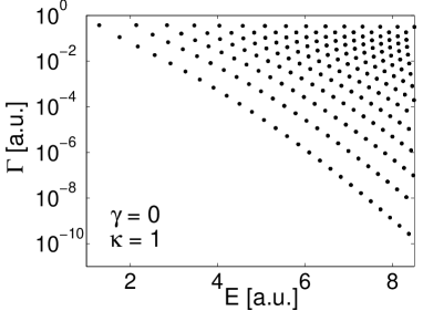
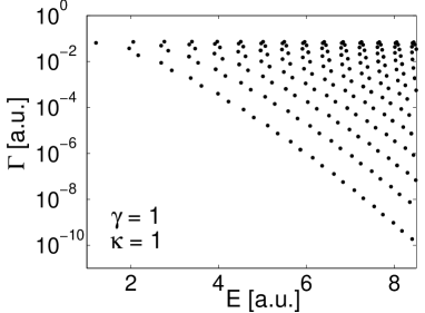
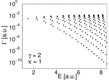
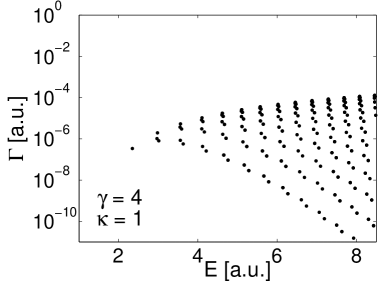
Figure 2: Energies $E$ and decay widths $\Gamma$ (logarithmic scale) for resonances in a magnetic guide for $\kappa=1$. An increasing Ioffe field strength leads to a global decrease of the decay widths and therefore has a stabilizing effect. At the same time the resonance pattern becomes distorted and a regrouping of the resonances into pairs is observed.

For $\gamma=0$ one observes a regular pattern for the arrangement of the complex energies, i.e. they are located along lines in the semi-logarithmic representation. This implies that the decay width essentially decreases exponentially with increasing energy along the mentioned lines. The decay width of the lowest (and here also broadest) resonance is $\Gamma^{\gamma=0}_{\text{min}}=0.3738$. Increasing $\gamma$ results in a distortion of the regular pattern. One observes the formation of vertical lines together with a regrouping of the resonances into pairs for larger $\gamma$ (see in particular figure 2 for $\gamma=4$). Here states with large decay widths are affected more strongly than long lived states. Overall we encounter a decrease of the decay width if $\gamma$ increases. Thus as it is well-known an additional Ioffe field has a stabilizing effect. For the decay widths of the lowest resonance state our calculation yields the series $\Gamma^{\gamma=1}_{\text{min}}=0.0648$, $\Gamma^{\gamma=2}_{\text{min}}=3.08\cdot 10^{-3}$, $\Gamma^{\gamma=4}_{\text{min}}=3.38\cdot 10^{-7}$ and $\Gamma^{\gamma=5}_{\text{min}}=1.04\cdot 10^{-9}$. These values suggest an exponential decrease of the decay widths if $\gamma$ increases. This agrees with the results of Sukumar and Brink who have estimated an exponential increase of lifetimes with growing Ioffe field strength by an analytical calculation Sukumar97 .

In Sec. III we have pointed out the degeneracy of the $\kappa=1$- and $\kappa=-1$-subspaces. For $\gamma\neq 0$ these degeneracies are expected to split up since the symmetry properties of the system changes. Figure 3 shows the resonances for $\gamma=1$. States belonging to the $\kappa=1$ or $\kappa=-1$ subspaces are indicated by a dot or cross, respectively.

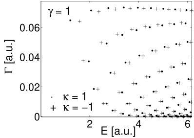
Figure 3: Resonance energies and decay widths in the $\kappa=1$- or $\kappa=-1$-subspaces at $\gamma=1$ (linear scale plot). Due to the finite Ioffe field formally degenerate pairs split up. States with negative quantum number $m$ are shifted towards higher resonance energies and vice versa. The splitting decreases with decreasing decay width.

Each state is accompanied by its degenerate partner for $\gamma=0$. The respective energy splitting decreases with decreasing decay width. In the following we will find that a small decay width is associated to the $\Lambda_{z}$ eigenvalue property of a resonance state: States with a small value for $\Gamma$ are localized far away from the center of the guide. Here the quadrupole field dominates the homogeneous Ioffe field and determines the appearence of the spectrum. Therefore these states become less affected by the Ioffe field which results in a decrease of the energy splitting.

Let us compare our results to those given by Hinds and Eberlein in Ref. Hinds00E . First of all we remark that we have studied a significant larger number of resonances.

	$m=\frac{1}{2}$		$m=\frac{3}{2}$
	$E$	${\Gamma}$	$E$	${\Gamma}$
	1.2937	0.3738	1.7591	0.1122
0	1.32	0.34	1.765	0.11
	2.1404	0.3788	2.5144	0.1444
1	2.125	0.34	2.52	0.15
	2.8438	0.3726	3.1711	0.1594
2	2.81	0.34	3.17	0.18

Table 4: Comparison between our results (bold face) and those obtained by Hinds and Eberlein for the first $3$ energetically lowest resonances in the $m=\frac{1}{2}$ and $m=\frac{3}{2}$ subspaces.

In table 4 we have listed the resonance energies and decay widths of the first $3$ states inside the $m=\frac{1}{2}$ and $m=\frac{3}{2}$ subspaces. Both results agree within a few percent. The difference might originate from the complicated procedure employed by Hinds and Eberlein to locate the resonance energies .

V.2 Dependence of the resonance energies on the eigenvalue of $\Lambda_{z}$

In this section we analyze how the energies and decay widths of the resonances are related to the eigenvalues of the angular momentum operator $\Lambda_{z}$. Although $\Lambda_{z}$ is a conserved quantity we have employed a set of basis functions which do not respect this fact. Thus we need to calculate the matrix element $m=\left<E,\kappa\right|\Lambda_{z}\left|E,\kappa\right>$ to receive the $\Lambda_{z}$-eigenvalues of the resonances. In order to do this one has to respect the non-Hermitian character of the Hamiltonian (19) which requires a complex symmetric scalar product. For a detailed discussion see Ref. Moiseyev98 .

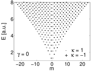
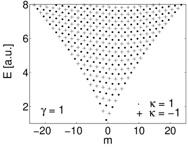
Figure 4: Resonance energies and $\Lambda_{z}$ eigenvalues of resonances for $\gamma=0$ (left picture) and $\gamma=1$ (right picture). For $\gamma=0$ the energies of the resonances form a symmetric pyramid-like pattern. For finite Ioffe field strength the pattern becomes asymmetric.

Figure 4 depicts the energies $E$ and the $\Lambda_{z}$ eigenvalue of the resonances. For $\gamma=0$ one observes each state to possess a degenerate counterpart, i.e. a state with opposite $m$. This results in the formation of a symmetric pyramid-like distribution where the maximum $\Lambda_{z}$ eigenvalue depends approximately linear on the resonance energy $E$. With increasing $\gamma$ the resonance energies in general are shifted towards larger values (this can hardly be seen in figure 4 for $\gamma=1$). Thereby, states with positive $m$ acquire a larger energetical shift than states with negative values of the quantum number $m$. Due to this asymmetric energy shift the distribution becomes asymmetric (with respect to $m\rightarrow-m$), too. Here energies of states having the same $\kappa$ quantum number form continuous, nearly horizontal, lines whereas we observe the resonance energies for $\gamma=0$ to be arranged on broken horizontal lines. In subsection V.4 we will show that in the limit of $\frac{\rho^{2}}{\gamma^{2}}\rightarrow 0$ one finds a pattern of equidistant straight horizontal lines formed by the resonance energies. Subsequent lines belong to states with opposite $\Sigma_{z}$ quantum number. With increasing $m$ values the states become less affected by the Ioffe field. Their wavefunctions become located farther away from the center of the guide. In this region the strength of the linearly increasing quadrupole field outweighs the effects of the Ioffe field.

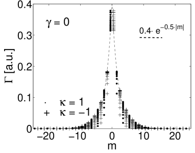
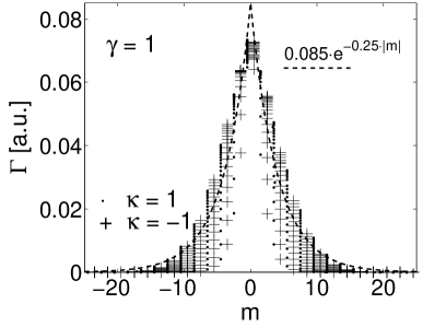
Figure 5: Decay widths and $\Lambda_{z}$ eigenvalues of resonances for $\gamma=0$ (left picture) and $\gamma=1$ (right picture). The decay width decreases exponentially with increasing modulus of $m$. With increasing Ioffe field strength one observes an overall decrease of the decay widths and a widening of the distribution.

In figure 5 the dependence of the decay widths on the $\Lambda_{z}$ eigenvalue is presented. Here we encounter an exponential decrease of the decay widths with increasing modulus of $m$. Overall the decay widths decrease if $\gamma$ increases and at the same time the distribution becomes broader.

V.3 Quasi-bound states for $\gamma=0$

Although a spin in our field configuration does not possess bound states there exist resonances with very long lifetimes, i.e. very small decay widths. The discussion of these quasi-bound states is the subject of the present section.

Transforming the Hamiltonian (7) to polar coordinates $(\rho,\phi)$ and exploiting the conservation of $\Lambda_{z}$ yields

$$H_{m}=\left<m\right|H\left|m\right>=\frac{1}{2}\left[-\frac{\partial^{2}}{\partial\rho^{2}}-\frac{1}{\rho}\frac{\partial}{\partial\rho}+\frac{\left(m+\frac{1}{2}\sigma_{z}\right)^{2}}{\rho^{2}}+\rho\sigma_{x}\right].$$ (28)

Performing the spin-space transformation

$$U=\frac{1}{\sqrt{2}}\left(\begin{array}[]{cc}1&1\\ 1&-1\\ \end{array}\right)$$ (31)

and introducing the spinor $\left|\Psi\right>=\rho^{-\frac{1}{2}}\left|\Phi\right>$ the corresponding Schrödinger equation becomes

$$\frac{1}{2}\left[-\frac{\partial^{2}}{\partial\rho^{2}}+\frac{m^{2}+m\sigma_{x}}{\rho^{2}}+\rho\sigma_{z}\right]\left|\Phi\right>=E\left|\Phi\right>.$$ (32)

The transformation (31) diagonalizes the $\vec{\mu}{\vec{B}}$ interaction term but leads to off-diagonal elements in the angular momentum term. In the limit of large $m$ this coupling between the up and down components of $\left|\Phi\right>$ can be neglected:

$$\frac{m^{2}+m\sigma_{x}}{\rho^{2}}\rightarrow\frac{m^{2}}{\rho^{2}}$$ (33)

which yields

$$\frac{1}{2}\left[-\frac{\partial^{2}}{\partial\rho^{2}}+\frac{m^{2}}{\rho^{2}}+\rho\sigma_{z}\right]\left|\Phi\right>=E_{qb}\left|\Phi\right>.$$ (34)

By construction this radial Schrödinger equation (34) does not couple the up- and down-component of the spinor wavefunction $\left|\Phi\right>$. The lower component is unbound since the corresponding effective potential is $V^{-}\left(\rho\right)=\frac{m^{2}}{2\rho^{2}}-\frac{1}{2}\rho$. In contrast to this the potential for the upper component is $V^{+}\left(\rho\right)=\frac{m^{2}}{2\rho^{2}}+\frac{1}{2}\rho$ and therefore bound solutions are allowed. We will refer to the corresponding states as the quasi-bound states $\left|\chi\right>=\left(\chi\left(\rho\right),0\right)^{T}$ which are described by the Schrödinger equation

$$\frac{1}{2}\left[-\chi^{\prime\prime}+\frac{m^{2}}{\rho^{2}}\chi+\rho\chi\right]=E_{qb}\chi.$$ (35)

Here a prime denotes the derivative with respect to $\rho$. In order to solve equation (35) we have utilized the FEMLAB software package wich employs the finite element method for solving differential equations .

		0	1	2	3	4	5
	$E$	1.2937	2.1404	2.8438	3.4688	4.0419	4.5769
$m=\frac{1}{2}$	$E_{qb}$	1.2829	2.1287	2.8324	3.4579	4.0315	4.5669
	%	0.83	0.55	0.40	0.31	0.26	0.22
	$E$	3.2660	3.8412	4.3797	4.8889	5.3741	5.8392
$m=\frac{11}{2}$	$E_{qb}$	3.2542	3.8256	4.3612	4.8684	5.3522	5.8162
	%	0.36	0.41	0.42	0.42	0.41	0.39
	$E$	4.7847	5.2629	5.7230	6.1673	6.5977	7.0156
$m=\frac{21}{2}$	$E_{qb}$	4.7805	5.2577	5.7169	6.1602	6.5897	7.0068
	%	0.09	0.10	0.11	0.12	0.12	0.13
	$E$	6.0956	6.5208	6.9344	7.3375	7.7311	8.1160
$m=\frac{31}{2}$	$E_{qb}$	6.0934	6.5181	6.9313	7.3341	7.7273	8.1118
	%	0.04	0.04	0.04	0.05	0.05	0.05
	$E$	7.2790	7.6689	8.0505	8.4245	-	-
$m=\frac{41}{2}$	$E_{qb}$	7.2774	7.6671	8.0486	8.4224	8.7891	9.1492
	%	0.02	0.02	0.02	0.02	-	-

Table 5: Comparison of the resonance energies to the approximate energies $E_{qb}$ obtained from equation (34). The first six resonance energies $E$ for 5 selected values of the quantum number $m$ are provided. The rows labelled by ’%’ show the relative difference between $E$ and $E_{qb}$ in percent.

In table 5 the resonance energies $E$ obtained from the complex scaling calculation are compared to the approximate energies $E_{qb}$ resulting from equation (34). Even for $m=\frac{1}{2}$ we find a remarkable good agreement between $E$ and $E_{qb}$ although the validity of equation (34) is not justified since the off-diagonal coupling terms are of the same magnitude than the diagonal ones. With increasing $m$ the discrepancy of $E$ and $E_{qb}$ decreases as suggested by (33). The surprisingly good quality of the approximation can be explained by looking at how the bound solution $\left|\chi\right>=\left(\chi\left(\rho\right),0\right)^{T}$ and the unbound wavefunction $\left|\zeta\right>=\left(0,\zeta\left(\rho\right)\right)^{T}$ are coupled by the Schrödinger equation (32):

$$\frac{m}{2}\left<\chi\right|\frac{\sigma_{x}}{\rho^{2}}\left|\zeta\right>=\frac{m}{2}\int d\rho\,\chi^{*}\left(\rho\right)\frac{1}{\rho^{2}}\zeta\left(\rho\right)$$ (36)

From this expression one recognizes that transitions from the bound state $\left|\chi\right>$ to the unbound state $\left|\zeta\right>$ are going to happen essentially at the center of the guide. However, since $m$ can only adopt half-integer values the centrifugal barrier in equation (34) always persists. Thus both wavefunctions $\left|\chi\right>$ and $\left|\zeta\right>$ vanish for $\rho\rightarrow 0$. However, this is the only region where the operator $\frac{1}{\rho^{2}}$ contributes significantly. Hence we have $\left<\chi\right|\frac{\sigma_{x}}{\rho^{2}}\left|\zeta\right>\ll 0$ and thus there is only a small coupling between the bound and unbound solution. Therefore the resonance states are very well described by the solutions $\left|\chi\right>$ of equation (35). This also explains the long lifetime of states with high $m$ quantum numbers. Here the large angular momentum barrier prevents the coupling between the bound and unbound channel. The particles are then located between the classical turning points of the potential $V_{\text{qb}}(\rho)=\frac{m^{2}}{2\rho^{2}}+\frac{1}{2}\rho$ at a distance of approximately $\rho_{\text{min}}=\sqrt[3]{2\,m^{2}}$.

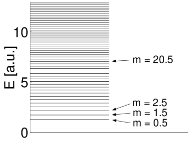
Figure 6: Energies $E_{\text{lr}}$ of the lowest resonances of each $m$ subspace calculated by using equation (37). Their accuracy is higher than the resolution of the plot.

Performing a harmonic approximation of the potential $V^{+}(\rho)$ around its minimum at $\rho_{\text{min}}$ yields a useful expression for the energy of the lowest resonance in each $\Lambda_{z}$ subspace

$$E_{\text{lr}}=\frac{\sqrt{3}}{2}\left(2\,m^{2}\right)^{-\frac{1}{3}}+\frac{3}{2}\left(\frac{m}{2}\right)^{\frac{2}{3}}.$$ (37)

This equation provides a very good approximation to the energies. The calculated resonance energies differ from the energies $E_{\text{lr}}$ by at most $0.05\%$. Figure 6 shows the energy spectrum obtained from equation (37). For large $m$ values the level spacing scales according to $m^{-\frac{1}{3}}$.

V.4 Quasi-bound states for $\gamma\neq 0$ and adiabatic approximation

In the previous section we have shown the existence of quasi-bound states in case of a vanishing Ioffe field. We will now show that similar states exist also if a Ioffe field is present. We start our investigation with the Hamiltonian

$$H_{m}=\left<m\right|H\left|m\right>=\frac{1}{2}\left[-\frac{\partial^{2}}{\partial\rho^{2}}-\frac{1}{\rho}\frac{\partial}{\partial\rho}+\frac{\left(m+\frac{1}{2}\sigma_{z}\right)^{2}}{\rho^{2}}+\rho\sigma_{x}+\gamma\sigma_{z}\right].$$ (38)

Introducing the spinor wavefunction $\left|\Psi\right>=\rho^{-\frac{1}{2}}\left|\Phi\right>$ and applying the unitary transformation

$$U=\frac{1}{\sqrt{2}}\left(\begin{array}[]{cc}\sqrt{1+\alpha}&\sqrt{1-\alpha}\\ \sqrt{1-\alpha}&-\sqrt{1+\alpha}\\ \end{array}\right)$$ (41)

with $\alpha=\frac{\gamma}{\sqrt{\gamma^{2}+\rho^{2}}}$ the corresponding Schrödinger equation becomes

$$\frac{1}{2}\left[-\frac{\partial^{2}}{\partial\rho^{2}}+\frac{m^{2}}{\rho^{2}}+\frac{m\alpha}{\rho^{2}}\sigma_{z}+\frac{\gamma}{\alpha}\sigma_{z}+\frac{\alpha^{4}}{4\gamma^{2}}-i\left(\frac{\alpha^{2}}{\gamma}\frac{\partial}{\partial\rho}-\rho\frac{\alpha^{4}}{\gamma^{3}}\right)\sigma_{y}+\frac{m\alpha}{\gamma\rho}\sigma_{x}\right]\left|\Phi\right>=E\left|\Phi\right>$$ (42)

Like without Ioffe field the unitarian (41) transforms the $\vec{\mu}\vec{B}$-coupling term into a diagonal form. However, unlike the transformation (31) $U$ in equation (41) depends explicitly on the coordinate $\rho$. Therefore the transformation of the derivative results in additional terms:

$$U^{+}\frac{\partial^{2}}{\partial\rho^{2}}U = U^{+}U^{\prime\prime}+2U^{+}U^{\prime}\frac{\partial}{\partial\rho}+\frac{\partial^{2}}{\partial\rho^{2}}.$$ (43)

Neglecting the off-diagonal coupling terms in equation (42) yields:

$$\frac{1}{2}\left[-\frac{\partial^{2}}{\partial\rho^{2}}+\frac{m^{2}}{\rho^{2}}+\frac{m\alpha}{\rho^{2}}\sigma_{z}+\frac{\gamma}{\alpha}\sigma_{z}+\frac{\alpha^{4}}{4\gamma^{2}}\right]\left|\Phi\right>=E_{qb}\left|\Phi\right>$$ (44)

Here similar to equation (34) only the upper component of the spinor $\left|\Phi\right>$ is bound. It obeys the Schrödinger equation

$$\frac{1}{2}\left[-\frac{\partial^{2}}{\partial\rho^{2}}+\frac{m^{2}}{\rho^{2}}+\sqrt{\gamma^{2}+\rho^{2}}+\frac{m\gamma}{\rho^{2}\sqrt{\gamma^{2}+\rho^{2}}}+\frac{\gamma^{2}}{4\left(\gamma^{2}+\rho^{2}\right)^{2}}\right]\chi=E_{qb}\chi.$$ (45)

		0	1	2	3	4	5
	$E$	2.8163	3.3978	3.9412	4.4547	4.9437	5.4123
$m=-\frac{1}{2}$	$E_{qb}$	2.8471	3.4272	3.9691	4.4813	4.9692	5.4369
	%	1.08	0.86	0.70	0.59	0.51	0.45
$l=0$	$E_{ad}$	2.8387	3.4205	3.9635	4.4764	4.9649	5.4329
	%	0.79	0.66	0.56	0.48	0.43	0.38
	$E$	4.4663	4.953	5.4199	5.8696	6.3045	6.7262
$m=\frac{11}{2}$	$E_{qb}$	4.4648	4.9514	5.4180	5.8677	6.3024	6.7240
	%	0.03	0.03	0.04	0.03	0.03	0.03
$l=6$	$E_{ad}$	4.4957	4.9797	5.4442	5.8921	6.3253	6.7457
	%	0.65	0.54	0.45	0.38	0.33	0.29
	$E$	6.8534	7.2540	7.6453	8.0280	8.4028	8.7703
$m=\frac{31}{2}$	$E_{qb}$	6.8523	7.2528	7.6440	8.0267	8.4014	8.7688
	%	0.02	0.02	0.02	0.02	0.02	0.02
$l=16$	$E_{ad}$	6.9044	7.3027	7.6918	8.0725	8.4455	8.8114
	%	0.74	0.67	0.60	0.55	0.51	0.47

Table 6: Comparison of the resonance energies to the approximate energies $E_{qb}$ and adiabatic energies $E_{ad}$ for $\gamma=5$. The first six resonance energies $E$ for 5 selected values of the $m$ quantum number are given. The rows labelled by ’%’ show the relative difference between $E$ and $E_{qb}$ or $E_{ad}$, respectively, in percent.

Table 6 compares the resonance energies $E$ obtained for $\gamma=5$ to the eigenvalues $E_{qb}$ calculated by solving the scalar radial Schrödinger equation (45). Apart from $m=-0.5$ the agreement is excellent with discrepancies lower than 0.05 %. This is again the result of a localization of the particle wavefunction away from center of the guide which is the only region where the off-diagonal coupling terms are remarkable. However, for $m=-0.5$ and $\gamma=5$ the effective potential of the Schrödinger equation (45) does not possess a centrifugal barrier. Here the wavefunction has non-zero contributions in the vicinity of the center of the guide. Hence the off-diagonal coupling terms of equation (42) become important. Considering the fact that the equation (45) here becomes certainly invalid the energies $E$ and $E_{qb}$ still agree surprisingly well (see table 6).

We now compare the results of the approximate Schrödinger equation (45) to those one would obtain within the so called adiabatic approximation. In this picture one assumes the projection of the atomic spin onto the local direction of the magnetic field to be conserved. Thus the coupling of the magnetic moment to the field reduces to $g\mu_{B}m_{S}\left|\vec{B}\right|$ with $m_{S}$ being the projection of the spin onto the local field direction. In case of a spin-$\frac{1}{2}$-particle in the magnetic guide the corresponding Hamiltonian becomes

$$H_{ad}=\frac{1}{2}\left[p_{x}^{2}+p_{y}^{2}\pm\sqrt{\gamma^{2}+x^{2}+y^{2}}\right]$$ (46)

having employed scaled coordinates (see Sec. II). Considering only the positive sign (which allows bound solutions) and introducing the wavefunction $\left|\Psi_{ad}\right>=\rho^{-\frac{1}{2}}\left|\Phi_{ad}\right>$ the corresponding Schrödinger equation becomes

$$\frac{1}{2}\left[-\frac{\partial^{2}}{\partial\rho^{2}}+\frac{l^{2}-\frac{1}{4}}{\rho^{2}}+\sqrt{\gamma^{2}+\rho^{2}}\right]\left|\Phi_{ad}\right>=E_{ad}\left|\Phi_{ad}\right>.$$ (47)

Here $l$ is the quantum number of the operator $L_{z}$ which is conserved due to the rotational invariance of the system around the $z$-axis. Note that unlike $m$ the quantum number $l$ is integer-valued. Table 6 shows a comparison of the adiabatic eigenvalues $E_{ad}$ to the exact resonance energies as well as the energies of the quasi-bound states $E_{qb}$. The quantum numbers $l$ and $m$ are chosen such that $l=m+\frac{1}{2}$. Only for $l=0$ or $m=-\frac{1}{2}$ the adiabatic energies $E_{ad}$ are in better agreement to the exact ones than the quasi-bound energies $E_{qb}$. One has to note that in contrast to $E_{ad}$ the energies $E_{qb}$ become exact in the limit of high $m$ quantum numbers. Moreover we have to emphasize that only the Schrödinger equation (45) yielding the quasi-bound states reproduces the correct degeneracies of the system. In contrast to this the corresponding adiabatic equation shows a two-fold degeneracy of the states $\left|l\right>$ and $\left|-l\right>$ for any value of $\gamma$.

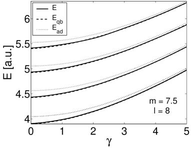
Figure 7: Comparison of the quasi-bound energies $E_{qb}$ and adiabatic energies $E_{ad}$ to the exact energies $E$. The figure shows the energies of the lowest four states in the $m=\frac{15}{2}$ and $l=8$ subspace, respectively. The discrepancy between $E$ and $E_{qb}$ is hardly visible throughout the complete $\gamma$-interval shown.

We now investigate how the different approximations perform for different $\gamma$ values. In figure (7) the energies obtained from each of the three methods (exact, quasi-bound, adiabatic) are depicted for the 4 energetically lowest resonances in the $m=\frac{15}{2}$ and $l=8$ subspace, respectively. One observes a remarkable agreement of $E$ and $E_{qb}$ throughout the complete $\gamma$-interval. In contrast to that severe discrepancies between the adiabatic and exact energies are revealed for small values of $\gamma$. This shows the extremely good performance of the quasi-bound approximation independently of the value of $\gamma$. This makes equation (45) the correct choice to calculate approximate eigenvalues.

Figure (7) also shows that if $\gamma$ becomes large the adiabatic approximation begins to perform well. In the limit of $\frac{\rho^{2}}{\gamma^{2}}\ll 1$ equation (47) can be further simplified. A series expansion of the potential term up to first order in $\frac{\rho^{2}}{\gamma^{2}}$ yields

$$\frac{1}{2}\left[-\frac{\partial^{2}}{\partial\rho^{2}}+\frac{l^{2}-\frac{1}{4}}{\rho^{2}}+\frac{\rho^{2}}{2\gamma}+\gamma\right]\left|\Phi_{ad}\right>=E_{ad}\left|\Phi_{ad}\right>.$$ (48)

This is the Schrödinger equation of a radial harmonic oscillator. The corresponding eigenenergies are given through

$$E_{nl}=\frac{\gamma}{2}+\sqrt{\frac{1}{2\gamma}}\left(2n+\left|l\right|+1\right).$$ (49)

Introducing the frequency $\omega=\sqrt{\frac{1}{2\gamma}}$ together with the substitution $l=m+\frac{1}{2}$ one arrives at the formula

$$E_{nm}=\frac{\gamma}{2}+\omega\left(2n+\left|m+\frac{1}{2}\right|+1\right).$$ (50)

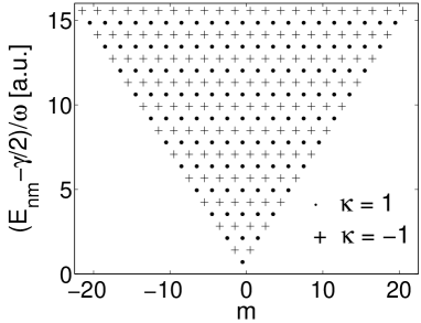
Figure 8: Graphical representation of the eigenenergies (50). The values of the quantum number $\kappa$ are calculated using equation (14). A pattern of equidistant horizontal lines with alternating $\kappa$ values is formed.

Figure 8 shows a plot of the energies $E_{nm}$. The corresponding $\Sigma_{z}$-eigenvalues are calculated using equation (14). The resultant pattern is similar to the one we have already observed in figure 4b. We find alternating equidistant horizontal lines of energies belonging to states of the two different $\Sigma_{z}$-subspaces.

V.5 Resonance energies and decay widths of ${}^{6}\text{Li}$ in the $2\,^{2}\text{S}_{\frac{1}{2}}\,,\,\text{F}=\frac{1}{2}$ hyperfine ground state

In order to experimentally prepare a magnetic guide one can superimpose the magnetic field of a current carrying wire by a so-called bias field oriented perpendicular to the current flow Folman02 . The resulting magnetic field possesses a line of zero field strength at a distance $\rho_{0}=\frac{\mu_{0}I}{2\pi B_{B}}$ parallel to the wire. A series expansion of the field around $\rho_{0}$ yields

$$\vec{B}\approx\frac{B_{B}}{\rho_{0}}\left(\begin{array}[]{c}x\\ -y\\ 0\\ \end{array}\right)+\frac{B_{B}}{\sqrt{2}\rho_{0}^{2}}\left(\begin{array}[]{c}-x^{2}+2xy+y^{2}\\ x^{2}+2xy-y^{2}\\ 0\\ \end{array}\right)+\frac{B_{B}}{\rho_{0}^{3}}\left(\begin{array}[]{c}y\left(y^{2}-3x^{2}\right)\\ -x\left(x^{2}-3y^{2}\right)\\ 0\\ \end{array}\right).$$ (60)

These are the quadrupolar, hexapolar and octopolar components of the field. As long as $\rho_{0}\gg 1$ one can neglect the higher order terms ending up with equation (4) for $B=0$. The gradient $b=\frac{2\pi B^{2}_{B}}{\mu_{0}I}$ is fully determined by the strength $B_{B}$ of the bias field and the current $I$.

For our discussion we choose the experimental parameters $I=2\,A$ and $B_{B}=10^{-2}T$. These are typically achievable values which are used for realizing magnetic microtraps. For this setup one finds the line of vanishing field strength at a distance $\rho_{0}=40\mu m$ above the wire. The gradient $b$ evaluates to $b=250\frac{T}{m}$. For the Landé-factor of ${}^{6}\text{Li}$ in its ground state ($2\,^{2}\text{S}_{\frac{1}{2}},\text{F}=\frac{1}{2}$) one obtains $g=|g_{F}|=|-\frac{2}{3}|$. Together with the mass $M=10964.67m_{e}$ the energy and the length scale become $\frac{1}{M}\left(\frac{bgM}{2}\right)^{\frac{2}{3}}=0.864\cdot 10^{-9}eV$ and $\left(\frac{bgM}{2}\right)^{-\frac{1}{3}}=89.63nm$, respectively. The resonance energy of the ground state is $E=1.12neV$ which corresponds to a temperature of $12.97\mu K$. This temperature regime is certainly accessible by todays cold atom experiments. Correspondingly the transition frequencies to excited states lie in the MHz regime. The lifetime of the ground state evaluates to $2.04\mu s$. Under consideration of the exponential scaling with increasing angular momentum almost arbitrarily long lifetimes can be achieved by preparing the atoms in high $\Lambda_{z}$ eigenstate, e.g. the minimum lifetime for a state with $|m|=\frac{41}{2}$ is $46.61s$.

VI Conclusion and Outlook

We have investigated the motion of a neutral spin-$\frac{1}{2}$-fermions in a magnetic quadrupole guide. The impact of an additionally applied homogeneous Ioffe field is also studied. Introducing a canonical scaling transformation of the phase space coordinates we have derived an effective two-dimensional Hamiltonian depending on a single parameter $\gamma$. The energies and decay widths of resonance states of the Schrödinger equation have been calculated by employing the complex scaling method. Utilizing a 2-dimensional harmonic oscillator basis we were able to converge hundreds of resonance states.

The analysis of the underlying Hamiltonian revealed a large number of symmetries. In the absence of a homogeneous Ioffe field we have found $15$ discrete symmetries of both unitary and anti-unitary character in addition to the conserved quantity $\Lambda_{z}=L_{z}-S_{z}$. A deeper investigation of the underlying symmetry group revealed a two-fold degeneracy of any energy level. If a Ioffe field is applied $\Lambda_{z}$ is still conserved but only 7 discrete symmetries remain. Due to the altered symmetry group the degeneracies are lifted.

We have calculated the resonance energies for several values of the parameter $\gamma$. A comparison to the values obtained by Hinds and Eberlein (Ref. Hinds00E ) has been performed. For $\gamma=0$ (vanishing Ioffe field) the resonance energies and decay widths form a regular pattern in the $E-\Gamma$ plane. Increasing the Ioffe field leads to a distorted distribution and the decay widths are pushed towards larger values. Thus the stability of the resonance states increases with the Ioffe field strength. An analysis of the lowest resonance has shown an exponential increase of lifetimes which agrees with results obtained by others Sukumar97 . Furthermore we could show an exponentially increasing lifetime with increasing modulus of the $m$ quantum number. Apparently, with increasing $|m|$ the wavefunctions become localized farther from the center of the guide where transitions to continuum states are induced.

We could show the existence of so called quasi-bound states which can be described by a scalar radial Schrödinger equation. The approximate eigenenergies agree very well with the resonance energies obtained from the complex scaling calculation and become exact in the limit of high $m$ quantum numbers. But even for low angular momenta an astonishing agreement could be observed. For $\gamma=0$ (without Ioffe field) this is due to the fact that $m$ is half-integer valued which leads to a non-vanishing angular momentum barrier. This prevents the particle from entering the center of the guide. However, the coupling matrix element to the unbound states does only assume significant values for $\rho\rightarrow 0$ i.e. the corresponding transitions are strongly inhibited. For $\gamma=0$ we have also calculated an analytic expression for the ground state energy in each $m$ subspace. For $\gamma\neq 0$ the quasi-bound energies are compared to those obtained from the so-called adiabatic approximations. We have shown that our approach is in general more accurate and reproduces in particular underlying degeneracies.

The results have been applied to the case of ${}^{6}\text{Li}$ in the $F=\frac{1}{2}$ state. Here we have considered a magnetic guide generated by a current carrying wire together with a homogeneous bias field. We have shown that for typical experimental parameter values the ground state energy corresponds to a temperature of a few micro-Kelvin. The lifetime of the resonance states can be extended up to minutes if the atoms are prepared in a sufficient high angular momentum state.

References

- (1) R. Folman et al, Adv. At. Mol. Opt. Phys. 48, 263 (2002)
- (2) C. J. Pethick and H. Smith, Bose-Einstein Condensation in Dilute Gases, Cambridge University Press (2002)
- (3) F. Schreck et al, Phys. Rev. Lett. 87, 080403 (2001)
- (4) T. H. Bergeman et al, J. Opt. Soc. Am. B, 2249 (1989)
- (5) K. Berg-Sorensen et al, Phys. Rev. A 53, 1653 (1996)
- (6) L. Vestergaard Hau, J. A. Golovchenko, and Michael M. Burns , Phys. Rev. Lett. 75, 1426 (1995)
- (7) J. P. Burke, Jr., Chris H. Greene, and B. D. Esry, Phys. Rev. A 54, 3225 (1996)
- (8) E. A. Hinds and C. Eberlein, Phys. Rev. A 61, 033614 (2000)
- (9) E. A. Hinds and C. Eberlein, Phys. Rev A 64, 039902(E) (2000)
- (10) R. M. Potvliege and V. Zehnlé, Phys. Rev. A 63, 025601 (2001)
- (11) R. Blümel,K. Dietrich , Phys. Rev. A 43, 22 (1991)
- (12) I. Lesanovsky, J. Schmiedmayer and P. Schmelcher, preprint
- (13) N. Moiseyev , Phys. Rep. 302, 5-6 (1998)
- (14) W. P. Reinhardt, Ann. Rev. Phys. Chem. 33, 223-55 (1982)
- (15) C. V. Sukumar and D. M. Brink, Phys. Rev. A 56, 2451 (1997)
- (16) T. Bergeman, G. Erez, and H. J. Metcalf, Phys. Rev. A 35, 1535 (1987)