Anharmonic Force Fields and Thermodynamic Functions using Density Functional Theory

Abstract

The very good performance of modern density functional theory for molecular geometries and harmonic vibrational frequencies has been well established. We investigate the performance of density functional theory (DFT) for quartic force fields, vibrational anharmonicity and rotation-vibration coupling constants, and thermodynamic functions beyond the RRHO (rigid rotor-harmonic oscillator) approximation of a number of small polyatomic molecules. Convergence in terms of basis set, integration grid and the numerical step size for determining the quartic force field by using central differences of analytical second derivatives has been investigated, as well as the performance of various exchange-correlation functionals. DFT is found to offer a cost-effective approach with manageable scalability for obtaining anharmonic molecular properties, and particularly as a source for anharmonic zero-point and thermal corrections for use in conjunction with benchmark ab initio thermochemistry methods.

I Introduction

The Kohn-Sham formulation of Density Functional Theory (DFT) is nowadays a commonly used tool in computational chemistry, being frequently applied to thermodynamics, structures, harmonic frequencies of various chemical compounds. Despite its successes in the accurate prediction of most ground-state and some excited state properties of molecules, its usefulness for calculating anharmonic force fields is less firmly established.

Anharmonic force fields allow direct comparison between computed and observed spectroscopic transitions, as opposed to comparing computed harmonic apples with observed anharmonic oranges, all the while making ‘hand-waving’ approximations about the importance of anharmonicity. The cost of high-quality ab initio anharmonic force field calculations rapidly becomes prohibitive as the number of atoms increases, and the relatively low cost of DFT calculations — as well as the fairly routine availability of analytical second derivatives — makes them attractive potential alternatives.

Until about two years ago, DFT anharmonic force field studies were rather scarce. Dressler and Thiel studied H₂O, F₂O, and CH₃F using several generalized gradient approximation (GGA) functionalsthiel . Detailed studies had been done for diatomicsHassanzedeh ; Sinnokrot , with the respective authors claiming very high accuracy. Concerning larger molecules, the full quartic force field of ammoniaanharmhandy1 , benzeneanharmhandy2 and diazomethaneBaraille have been studied with a hybrid density functional.

In the last couple of years, an increasing number of anharmonic force fields using density have been published and several groups have been working on this subject. Noteworthy are the activities in the Handy group with studies of furan, pyrrole and thiopheneRudolf and phosphorus pentafluorideTew , which in fact yielded even more accurate results on these medium-sized organic systems than suggested by the small-molecule validation studies cited above. In addition to this, the group of HessNeugebauer (using the B3LYPB3LYP and BP86BP86 functionals) and BaroneBaroneval (using B3LYP) have published validation studies on a small number of mainly triatomic molecules. Furthermore, two of us published a detailed study on the azabenzene series, also exploring the possibility of combining DFT anharmonic force fields with coupled cluster geometries and harmonic frequenciesAzabenzenes . Barone carried out a similar study on the azabenzenes using a different functional and basis setBaroneAzabenzenes .

Another potential application of interest concerns high-accuracy computational thermochemistry. Computed molecular atomization energies require zero-point vibrational energies (ZPVEs) and thermal corrections. As molecules grow, ZPVEs make up an increasingly important part of the molecular binding energy — e.g., 62.08 kcal/mol in benzenebenzeneW2 — and approximations about the anharmonic contribution to the ZPVE introduce ever larger sources of potential error. This issue becomes especially acute with nonempirical extrapolation-based methods like W1, W2, and W3 theoryW2 ; W3 or explicitly correlated methods like CC-R12KlopperReview , which can fairly routinely yield atomization energies to sub-kcal/mol accuracy. Thermal corrections at room temperature can reasonably be expected to be reproduced fairly well for semirigid molecules, but in applications where high-temperature data are important (e.g., combustion modeling), vibrational anharmonicity, rovibrational coupling, and centrifugal distortion significantly affect thermodynamic functions (see, e.g., Refs.h2o ; cf2 ). All the required molecular properties can be readily obtained by vibrational perturbation theory when calculating the quartic force field of the respective compoundrovib1 ; rovib2 ; rovib3 ; rovib4 ; rovib5 .

Since the computation of a quartic force field using density functional theory is unlikely to require more computer time than W$n$ or explicitly correlated methods, it could become a routine step in such studies. It was previously shownW2book that the use of accurate ZPVEs from large-scale ab initio anharmonic force field calculations, instead of scaled B3LYP/cc-pVTZ harmonic frequencies, improved the mean absolute error of W2 theory over the W2-1 set of 28 small molecules (with very precisely known experimental binding energies) from 0.30 to 0.23 kcal/mol, and the maximum absolute error from 0.78 to 0.64 kcal/mol. This can be compared to the error when including up to connected quadruple excitations in the extrapolation scheme, where the mean absolute error (over a sample additionally including some molecules beset with nondynamical correlation) is reduced from 0.40 (W2) to 0.22 (W3) kcal/mol.

Assuming that we would like to achieve the best accuracy possible, we ought to be able to mitigate the error introduced by the ZPVE by using quartic DFT force fields to calculate the anharmonic corrections.

Of course, other approaches than vibrational perturbation theory could be used in conjunction with density functional methods, such as the VSCF-CC methodGerber1 ; Gerber2 ; Gerber3 ; Gerber4 ; Hirao1 ; Christiansen . However, as these methods are presently $J=0$ (i.e., rotational ground state) methods, the effects of rovibrational coupling and centrifugal distortion on the thermodynamic functions would have to be neglected.

In the present work, we report on a detailed validation study of DFT methods for all these properties, and will consider the dependence of their accuracy on the exchange-correlation functional, the basis set, the quality of the numerical integration grid, and the step size used in numerical differentiation.

II Computational Details

Following the approach first proposed by Schneider and Thielrovib4 , a full cubic and a semidiagonal quartic force field are obtained by central numerical differentiation (in rectilinear normal coordinates about the equilibrium geometry) of analytical second derivatives. The latter were obtained by means of locally modified versions of gaussian 98g98 ; modified routines from cadpacCadpac were used as the driver for the numerical differentiation. routine. In this approach, the potential energy surface is expanded through quartic terms at the global minimum geometry like:

$$V=\frac{1}{2}\sum_{i}\omega_{i}q^{2}_{i}+\frac{1}{6}\sum_{ijk}\phi_{ijk}q_{i}q_{j}q_{k}+\frac{1}{24}\sum_{ijk}\phi_{ijkk}q_{i}q_{j}q_{k}q_{l}$$ (1)

where the $q_{i}$ are dimensionless rectangular normal coordinates, $\omega_{i}$ are harmonic frequencies, and $\phi_{ijk}$ and $\phi_{ijkl}$ third and fourth derivatives with respect to the $q_{i}$ at the equilibrium geometry.

All the force fields have been analyzed by means of the spectroSpectro and polyadPolyad rovibrational perturbation theory programs developed by the Handy and Martin groups, respectively.

In all cases, when strong Fermi resonances lead to band origins perturbed more than about 2 cm^-1 from their second-order position, the deperturbed values are reported and resonance matrices diagonalized to obtain the true band origins. Rotational constants were similarly deperturbed for strong Coriolis resonances.

Thermodynamic functions beyond the harmonic approximation are obtained by means of the integration of asymptotic series method as implemented in the NASA PAC99 program of McBride and GordonPAC99 .

III Results and discussion

To avoid issues with experimental data, such as problems with the assignment of the spectra as has been reported in our previous studyAzabenzenes , we decided to solely compare our results to ab initio (coupled cluster) data of quartic force fields which have been published for molecules with more than two atoms. Here, 17 molecules, namely C₂H₂c2h2 , C₂H₄c2h4 , CCl₂, CF₂cf2 , CH₂NHch2nh , CH₂ch2 , CH₄ch4 , H₂COh2co , H₂Oh2o , H₂Sh2s , HCNhcn , N₂On2o , NH₂nh2 , PH₃ph3 , SiF₄sif4 , SiH₄sih4 , and SO₂so2 , have been included with some of the older data being recalculated with a more extended basis set.

III.1 Numerical quadrature

First of all, we have to investigate the dependence on the integration grid. We shall restrict ourselves to the HCTH/407 functionalHCTH407 , using a TZ2P basis set for the H₂O, SO₂ and N₂O molecules together with a step size of 0.02 a.u. for the central differences. The grids considered here are direct products of Euler-Maclaurin radial gridsHan93 ranging from 75 to 400 points, with Lebedev angular gridsLebedev ranging from 194 to 974 points. In addition, we considered some ‘pruned’ grids, in which the radial coordinate is divided into five zones (inner core, inner valence, valence, outer valence, and long-range) and different angular grid densities are used for each zone. The ‘SG1’, ’Medium’, ’Fine’, and ’Ultrafine’ standard grids in gaussian 9x correspond to pruned (50,194), (75,194), (75,302), and (99,590) grids, respectively. Inter-atom partitioning was done according to Ref.SSF .

Let us first consider the error in the off-diagonal stretching anharmonicity, relative to our largest grid (unpruned 400$\times$974). Unfortunately, sizable errors are seen for the standard gaussian-type grids, both due to their small intrinsic size and to the pruning. Hence, they cannot be recommended for this type of calculation, since these values are quite significant for the calculation of the thermodynamic functions and fundamental frequencies. The results are shown in Figure 1a to Figure 1c. As it is apparent from these figures, a very large number of radial grid points is needed for the accurate description of the quartic force field. From the values in Figure 1, we conclude that a 200$\times$974 grid for our calculations if the molecules include only first-row atoms, and the 300$\times$974 grid otherwise will be sufficient. We modified the code to add two additional pruned grids, 140$\times$974 and 199$\times$974 (which are invoked by new keywords ’Grid=Huge’ and ’Grid=Insane’, respectively). For these intrinsically finer-meshed grids, pruning deteriorates numerical precision less, and if 1 cm^-1 precision is sufficient, the ‘Huge’ grid will be generally adequate for first-row, and the ‘Insane’ grid for second-row molecules.

Unfortunately, Gaussian does permit using different radial grids on different atoms, although such variation can be somewhat simulated by manipulation of the pruning zone boundaries. It is however possible to use a different (coarser) grid in the CPKS (coupled-perturbed Kohn-Sham) steps, and here we were able to reduce grid size to as small as SG1 (i.e., pruned 75$\times$194), thus reducing overall computational cost. For instance, for methylene imine CH₂NH, this approximation reduced CPU time by half, while the computed fundamental frequencies change by less than 0.2 cm^-1. The importance of using a very large energy+gradients grid is apparent for this molecule as well: Even a relatively large 99$\times$590 (or in its pruned version, ‘Ultrafine’) grid will yield errors for some frequencies of more than 8 cm^-1, and the 140$\times$590 grid errors of 1 cm^-1. We expect similar behavior for other quantum chemical program systems, where grid sizes will likewise need to be increased well beyond what is normally required. Needless to say, errors are further exacerbated if one of the fundamentals affected by grid error is involved in a strong Fermi resonance. For example, in CH₂NH, the change in going from a pruned 75$\times$302 to an unpruned 140$\times$590 CPHF grid changes the eigenvalues of the fundamentals affected by Fermi resonances by about ten cm^-1. The deperturbed values, however, change by less than 0.5 cm^-1. Although this is clearly undesirable (and an inherent weakness of the method), in such a situation it becomes unclear which grid is actually the best to use, since even at large grid sizes the changes are significant.

III.2 Basis set

For the basis sets investigated, we have used Dunning’s cc-pV$n$Z and aug-cc-pV$n$Z correlation consistent basis sets for the first rowPVXZfirst , and the cc-pV($n$+d)Z and aug-cc-pV($n$+d)Z basis sets of Wilson, Peterson, and Dunning for the second row. (The latter include additional high-exponent $d$ functions, which have been shown to be importantso2 for spectroscopic constants of molecules in which a second-row atom is surrounded by one of more highly electronegative first-row atoms.) As for smaller basis sets, we considered the TZ2PTZ2P and DZP DZP basis sets. (Note that the TZ2P version used by most groups actually includes a third $d$ function for second-row atoms.) In all, we investigated the aug-cc-pVQZ, cc-pVQZ, aug-cc-pVTZ, cc-pVTZ, TZ2P and DZP basis sets, using the B97-1 hybrid functionalHCTH93 and a step size of 0.02 Bohr. Here, we compare to the largest basis set (aug-cc-pVQZ), which for DFT calculations of these properties is close to the Kohn-Sham basis set limit. In figure 2, now the mean errors of the zero-point energies are shown for the C₂H₄, H₂O, SO₂ and N₂O molecules, in addition to the overall error of the functional compared to coupled cluster data. The latter data shows when the basis error becomes significant enough to affect the error made by the functional itself. This happens only to the DZP basis set, although its overall mean error compared to the reference data is not larger than for the largest basis set employed. For the TZ2P basis, there seems to be some error compensation for this functional. Basically, the error made by the cc-pVTZ basis set is still very small compared to the aug-cc-pVQZ basis set, with the TZ2P basis set error still being significantly smaller than the functional error and the DZP basis set error being comparable. Thus, from these results, either the TZ2P or cc-pVTZ basis sets seem preferable, with the DZP basis set being an option for the very largest molecules.

III.3 Step size for numerical differentiation

As a third variable, an optimal numerical step size has to be determined. In a numerical derivatives calculation, it always represents a compromise between discretization error and roundoff error. All calculations have been done using an unpruned 200$\times$590 grid for CH₂NH, a molecule which proved to be very much affected by step size issues. For the first three modes, we compare to the deperturbed values to circumvent the difficulties mentioned above. In order to reduce roundoff error as much as possible, the KS and CPKS equations were basically converged to machine precision.

We considered five different approaches to the step size. All of them have been done along the unnormalized Cartesian displacement vectors of the mass weighted normal coordinates, such asGaussianpages :

$$\vec{r}=\vec{r}+q_{step}(i)\times\vec{l}$$ (2)

All stepsizes $q_{step}(i)$ are in $bohr\times amu$. In the first, a constant ‘one size fits all’ displacement was made in all modes:

$$q_{step}(i)=\hbox{constant}$$ (3)

In the second, we employed a variable step size proportional to the square root of the reduced mass for each particular vibration:

$$q_{step}(i)=\hbox{constant}\times\sqrt{\frac{\mu}{\hbox{amu}}}$$ (4)

This corresponds to normalising the displacement vector to have the same stepsize for different isotopes.

The third approach is to choose a step size such that within the harmonic oscillator approximation, the displacement in that particular mode causes a certain given energy change, e.g., 1 millihartree as in Ref.anharmhandy2

The fourth approach is to choose an unnormalised stepsize dependent on the force constant $k$. The is achieved by dividing through the reduced mass and the frequency of the corresponding mode:

$$q_{step}(i)=\hbox{constant}\times\frac{1}{\sqrt{\frac{\mu}{\hbox{amu}}}}\times\frac{1000~{}\hbox{cm}^{-1}}{\omega(i)}\propto\hbox{constant}\times\frac{1}{\sqrt{k}}$$ (5)

Finally, in the fifth approach we make the step size dependent on both the reduced mass and the absolute value of the harmonic frequency associated with the normal coordinate involved:

$$q_{step}(i)=\hbox{constant}\times\sqrt{\frac{\mu}{\hbox{amu}}}\times\sqrt{\frac{1000~{}\hbox{cm}^{-1}}{\omega(i)}}$$ (6)

Furthermore, in the absence of an analytical fourth derivatives code which would by definition render the ‘true’ answer, we can attempt determining the latter by means of Richardson extrapolationRalRab . At the lowest level, we combine two different step sizes h and 2h at the position x and reduce the error like:

$$D_{1}=\phi_{jjjj}(x)+O(h^{2})=\frac{\omega_{j}(x+h)+\omega_{j}(x-h)-2\omega_{j}(x)}{(h)^{2}}$$ (7)

$$D_{2}=\phi_{jjjj}(x)+O(4h^{2})=\frac{\omega_{j}(x+2h)+\omega_{j}(x-2h)-2\omega_{j}(x)}{(2h)^{2}}$$ (8)

and thus:

$$\frac{(4D_{1}-D_{2})}{3}=D_{1}+\frac{D_{1}-D_{2}}{3}=\phi_{jjjj}+O(h^{4})$$ (9)

This formula is actually equivalent to the use of a five-point fourth-order central difference formula. The Richardson approach can be applied recursively in order to minimize discretization error: with level $m$ estimates having an error term $O(h^{2m})$, the next level Richardson estimate $D^{[m]}_{1}+(D^{[m]}_{1}-D^{[m]}_{2})/(4^{m}-1)$ will have an error $O(h^{2m+2})$.

We have tightened convergence criteria at all stages of the electronic structure calculations to $10^{-10}$ or better (no convergence could be achieved with even tighter criteria). Yet even so, unacceptable roundoff error is introduced for small step sizes. As a result, Richardson extrapolation is only reliable for rather large step sizes, as can be seen in Table 1. The last column shows the most accurate values, combining the step sizes of 0.10, 0.12 and 0.14 bohr. Even when including the step size of 0.08 bohr (in column 8) into the formula, we probably see some roundoff error, explaining the (small) difference of up to 3 cm^-1 between both values — nevertheless, we expect the algorithm to be nearly converged. Comparing methods (1-5, method 1 with a stepsize of 0.025 Å), the maximum (mean absolute) errors compared to the last column (our reference, in fact) are 4 (1.6), 4 (1.2), 9 (4.0), 8 (2.1) and 1 (0.2) cm^-1. All methods (except method 3) have been calculated by finding an optimal constant stepsize prefactor, which is shown in the second line of Table 1. This constant prefactor is very important which becomes apparent when looking at mode 1 and mode 7 to 9 of method 1: For large frequencies (like mode 1), a small step size is needed as can be seen when comparing to the reference values. The error at 0.12 bohr for this mode will be as large as 30 cm^-1. On the other hand, a step size of 0.02 bohr yields errors of 50 cm^-1 for mode 7 and 30 cm^-1 for mode 8. The spurious interchange of fundamentals 8 and 9 at this step size could even lead to an incorrect assignment. Thus, the choice of step size is critical when calculating quartic force fields, and a worst-case error of about 5 cm^-1 still needs to be assumed even with all step size algorithms. These step size issues in fact transfer to $all$ molecules investigated, as we have done also with method (4). Here, the force fields are (compared to our reference coupled cluster values), as a rule of thumb, about twice as bad as when using method (5). The only fundamental remedy would be the calculation of third Kohn-Sham derivatives and taking numerical first derivatives of these, which to our knowledge has not been implemented in any quantum chemical code.

III.4 Exchange-correlation functionals

For assessing the different currently available density functionals for this problem, we employed several GGA functionals (BLYPBLYP , HCTH407HCTH407 , PBE PBE ) and hybrid density functionals (B3LYPB3LYP , B97-1HCTH93 , B97-2B97-2 , and PBE0PBE0 ). For all these functionals, we consider the full validation set of 17 molecules mentioned above.

For this purpose, we used both the TZ2P and cc-pVTZ basis sets to look at the performance of the functionals for the different basis sets. Although force fields for all the aforementioned molecules have been calculated with the two basis sets mentioned, the C₂H₂ molecule required diffuse functions to yield qualitatively correct bending anharmonicities. This is consistent with results obtained by ab initio correlation methods (which generate spurious positive anharmonicities with standard basis sets), whereas Hartree-Fock renders negative anharmonic corrections even without the use of diffuse functionsc2h2 . In all tables and figures, results for C₂H₂ thus refer to the aug-cc-pVTZ basis set. In the case of the symmetric tops CH₄, SiH₄ and SiF₄, we perturbed the masses of the hydrogens by 0.0001 atomic mass units in order to break symmetry. Here, Coriolis coupling between the now non-degenerate frequencies had to be taken into account. For CH₂, a quasi-linear molecule, both B97-1 and HCTH/407 yield positive anharmonic corrections when using the TZ2P basis set- those were the only calculations excluded from our evaluation. For CH₂NH, we were unable to use spectro due to the complicated resonances in this molecule (see Ref.ch2nh for a discussion) — the deperturbed values of the 9$\times$9 perturbation matrix from polyad were consistently used instead.

In figure 3, the RMS and mean absolute errors of the zero-point energies for all the molecules mentioned above are shown. Discussing the GGA functionals, HCTH/407 is a vast improvement over both PBE and BLYP, reducing their RMS error by almost a factor of two. Still, it is not quite comparable to the hybrid functionals, which render the lowest errors. The error in their zero-point energies is another factor of two lower than the one obtained by HCTH/407. The scaled B3LYP harmonic zero-point energy displays an error compared to HCTH/407. The error is about 0.33 kcal/mol, compared to 0.13 to 0.19 kcal/mol for the hybrid functionals. Here, B97-1 and B3LYP yield the lowest errors around 0.14 kcal/mol for both basis sets. For the cc-pVTZ basis set, all functionals yield a marginally worse zero-point energy compared to the TZ2P basis set. This is in line with our previous studies on geometriesBMH , where the combination of DFT/cc-pVTZ generally showed larger errors compared than DFT/TZ2P. Generally, the B3LYP functional returns results about 50% better than the ZPE determined by scaled B3LYP.

Discussing the fundamental frequencies in table 2, we can evaluate the accuracy of density functionals for the calculation of such properties which might prove useful when assigning experimental IR-spectra. All hybrid functionals yield RMS errors between 30 and 40 cm^-1 for the 103 frequencies investigated, with B97-1/TZ2P showing consistently the lowest errors. All pure GGA functionals underestimate both harmonic and fundamental frequencies by at least 25 cm^-1, casting doubt on any values computed by such methods. The difference between the errors of the calculated anharmonic and harmonic frequencies, shown in the first four columns, which are almost negligible and very large in comparison to those just done in the correction (last two columns). The latter emphasizes the agreement when using accurate harmonic frequencies from a higher level method such as CCSD(T). For such a combined method, the RMS errors are between 6 and 11 cm^-1, with surprisingly the hybrid functionals such as B97-1 and PBE0 having errors around 9 cm^-1 and HCTH/407 and BLYP around 6 cm^-1. In comparison, determining the anharmonic correction by simply scaling the harmonic frequency by a constant factor fails completely: Its RMS error is as large as for the fundamental frequencies itself.

As for the zero-point energies, HCTH/407 is slightly more accurate than the scaled B3LYP harmonic frequencies, and BLYP is somewhat less accurate than PBE for our validation set. Overall, we can expect an accuracy of about 30 cm^-1 or less when calculating fundamental frequencies for a diverse set of semirigid molecules using perturbation theory. This is much more than we would expect for organic moleculesAzabenzenes , but consistent with previous studies on a larger number of harmonic frequenciesBMK .

Returning to zero-point energies, these will be much improved when including harmonic frequencies at the reference level and just adding DFT anharmonic corrections. These errors are displayed in Figure 4, and can be readily compared to those obtained in Figure 3 (note the different scale of both figures). The error is reduced by at least a factor of five, showing the superiority of such a combined method. As for the anharmonic corrections, the GGA functionals BLYP and HCTH/407 yield the lowest errors, about reducing the errors of the hybrid functionals by 50%. In comparison, simply using the scaled B3LYP frequencies shows no improvement, as the RMS error would remain unchanged at 0.33 kcal/mol.

An additional observable obtained when calculating the anharmonic force field is the rotational constant. While A_e, B_e and C_e are only dependent on the electronic minimum geometry, the vibrationally averaged A₀, B₀ and C₀ are accessible by experiment. In Table 3, the mean and RMS errors (in %) for the 37 symmetry-unique rotational constants of the 16 molecules investigated are displayed. For the correction $A_{e}-A_{0}$ we chose not to report the errors in %, since the reference values are already very small and thus large relative errors are made by the functionals. As expected, the GGA functionals fare worse than the hybrid functionals with the exception of the HCTH/407 functional. This exceptional property of HCTH/407 has been reported beforeBMK ; tHCTH , with its geometry errors reduced by half in comparison to the other GGA functionals. For the hybrid functionals, the cc-pVTZ basis set gives lower errors than TZ2P, with the opposite for all GGA functionals. The accuracy of the hybrid functionals range from 0.06 to 0.13 cm^-1 (0.9 to 1.25 %) for $A_{e}$ and $A_{0}$. When only comparing the correction R_e-R₀ to these values, the error will be cut in half. This contrasts the RMS errors of the frequencies, where the anharmonic correction has an error which is about five times as low as the error of the frequency itself. Thus, adding the corrections for example to CCSD(T) structures will not be as rewarding as it was the case in the previous paragraph. As in Table 2 for the anharmonic corrections, all functionals now give quite similar errors.

III.5 Thermodynamic functions

Finally, we turn to thermodynamic functions evaluated by four different methods and compare them to our reference values. Since rotational and vibrational levels contribute to those, error cancellation can take effect here.

In Table 4 (method 1), the heat capacity, the difference of the enthalpy at a given temperature and the enthalpy at 0K, and the entropy are given at room temperature, 600 K and 2000 K. Whereas there is little difference between both basis sets, the functionals show the expected behavior, with the hybrid functionals and HCTH/407 giving quite similar errors. BLYP and PBE are again the worst performers, their errors being about twice as large. For the heat capacity, the initial error at 298.15 K is larger than the error at 600 K for all functionals, suggesting some error cancellation at this value.

The relative importance of various post-RRHO contributions at high temperature (say, 2000 K) varies somewhat with the molecule. For H₂O, vibrational anharmonicity and centrifugal stretching are about equally important, rovibrational coupling rather less so. For CH₂NH, vibrational anharmonicity predominates, with rovibrational coupling a distant second. For both C₂H₂ and N₂O, vibrational anharmonicity far outweighs the two other contributions. In SO₂ a balance between the three contributions prevails.

When applying the RRHO approximation using just harmonic frequencies and bottom-of-the-well rotational constants, as reported in Table 5 (method 2), somewhat surprising results are obtained: At low temperatures (room temperature), this method is easily competitive to calculating the full force field. In fact, most errors will be lower when using the RRHO approximation in conjunction with DFT for this temperatureTSEliot . Especially the errors of BLYP and PBE are reduced and comparable to the hybrid functionals for all temperatures. Again, there is barely any difference between the two basis sets. At 600 K, the entropy and enthalpy show the same behavior, only the heat capacity already has an error twice as high than when calculating the force field. At 2000 K, the errors of the RRHO approximation becomes quite large, with a factor of two (for the entropy) up to five (for enthalpy and heat capacity) between Table 4 and Table 5. Thus, when calculating such properties at room temperature, the error in the DFT method itself will be large compared to the error by making such an approximation. Taking just the coupled cluster frequencies and rotational constants from the reference method shows a similar behavior, with the errors naturally reduced in comparison to DFT by another factor of two for 298.15 K. At 600K, the error becomes already comparable to the one obtained by the best density functionals, and at 2000 K it is even higher in many cases.

Table 6 (method 3) represents a common compromise between the RRHO approximation and using the full scale quartic force field — especially when working from experimental data. Here, anharmonic frequencies and vibrationally averaged rotational constants are substituted in the RRHO approximation and all additional effects of anharmonicity, rovibrational coupling, and centrifugal stretching are neglected. At low temperatures, this method basically yields the same results as fully anharmonic calculations. The difference between both methods is less than 5% at room temperature and 600 K, with BLYP and PBE yielding again larger errors than the hybrid functionals. At 2000 K, however, neglecting these terms causes a large loss in accuracy, although the errors are not as large as when completely neglecting anharmonic effects. Still, the error in the heat capacity (normally the most sensitive quantity, as it involves the second moment of the partition function) is only lowered by about 20%, and the error of the entropy and enthalpy approximately by a third. Method 3 is thus an acceptable solution at low temperatures, and a stop-gap solution at elevated temperatures (around 600 K) when no quartic force field is available. By replacing the density functional values by the ones of our reference method, the error becomes much smaller. Again, an estimate can be made when this method becomes unreliable – this will be only at very large temperatures above 600 K. Of course, it requires the calculation of a full CCSD(T) force field which is done in our reference calculations, which would be prohibitive for many molecules.

Finally, the last method (4), shown in Table 7, includes all the effects covered in method 1, but in addition the equilibrium geometry and harmonic frequencies from the reference coupled cluster calculation were substituted in the rovibrational perturbation theory analysis. (This represents a hybrid approach in which a harmonic large basis set coupled cluster calculation would be combined with a DFT anharmonic force field.) Comparing the results to Table 4, especially at low temperatures an improvement is apparent. The initial error is reduced by a factor of two to three at room temperature. For larger temperatures, this improvement becomes visibly smaller, with the entropy the most affected variable by the change. At 2000 K, it is the only function showing a lower error than the one obtained by a pure DFT anharmonic force field. For both the heat capacity and the enthalpy, an error cancellation for DFT takes place, thus showing a lower error for method (1) than method (4). Comparing the functionals, only PBE gives somewhat worse results for this method. For the heat capacities and enthalpy at 298.15 and 600 K, the accuracy of this method can already be compared to the anharmonic CCSD(T) results obtained by method(3). The entropy, however will yield errors about four times as large at 298.15 K. This is of course the only method which yields a reasonable performance over the full temperature range.

IV Conclusions

In this validation study, we have calculated DFT anharmonic force fields for 17 small (triatomic and larger) molecules.

At least using the present approach (finite differences of analytical Hessians), we find anharmonicities to be very sensitive to the DFT integration grid, with grids as large as 140$\times$974 (first row) and 200$\times$974 (second row) being required for 1 cm^-1 numerical precision in fundamental frequencies.

The finite difference step sizes are another source of error. Either high-frequency or low-frequency modes are mainly affected, and too large or too small values will lead to large errors. Various adaptive-stepsize approaches yield satisfactory results.

Basis sets of at least TZ2P quality appear to be called for, although DZP quality may be an acceptable compromise for the very largest molecules.

HCTH/407 appears to be the most suitable GGA functional for the purpose, and B97-1 the most suitable hybrid functional, immediately followed by B3LYP. Somewhat surprisingly, when combining DFT anharmonicities with large basis set CCSD(T) geometries and harmonic frequencies, GGA functionals yield better results than their hybrid counterparts.

Fundamental frequencies can be determined to an accuracy of only 30 cm^-1, which is about the error that functionals also yield for harmonic frequencies. Of course, for organic molecules, this error will be reduced and DFT might prove useful in helping experimentalists in their assignments. For inorganic molecules, however, this accuracy might not be enough, and a higher level method will have to be used to calculate the harmonic frequencies.

The same applies to zero-point energies. DFT zero-point energies alone might not be accurate enough for using them as an addition to W2 or W3 theories, only in combination with e.g. CCSD(T) harmonic frequencies their values will get the desired error estimations. Since a full CCSD(T) force field with a sufficiently large basis set is so expensive, this might be an attractive alternative in many cases.

DFT may be useful in computing vibrational corrections to rotational constants obtained at higher levels of theory: the intrinsic errors in DFT rotational constants are large enough that they outweigh any advantage gained by the anharmonic computation.

DFT anharmonic force fields are useful in obtaining thermodynamic functions at elevated temperatures. At room temperature, the RRHO approximation is generally sufficient for semirigid molecules.

Finally, DFT-computed anharmonic corrections to the zero-point vibrational energy will somewhat enhance the reliability of high-level ab initio thermochemical data.

V Acknowledgments

ADB acknowledges a postdoctoral fellowship from the Feinberg Graduate School (Weizmann Institute). Research at Weizmann was supported by the Minerva Foundation, Munich, Germany, by the Lise Meitner-Minerva Center for Computational Quantum Chemistry (of which JMLM is a member), and by the Helen and Martin Kimmel Center for Molecular Design. This work is related to Project 2003-024-1-100, ”Selected Free Radicals and Critical Intermediates: Thermodynamic Properties from Theory and Experiment,” of the International Union of Pure and Applied Chemistry (IUPAC).

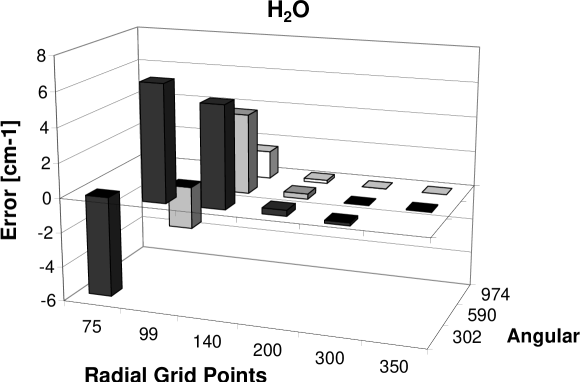
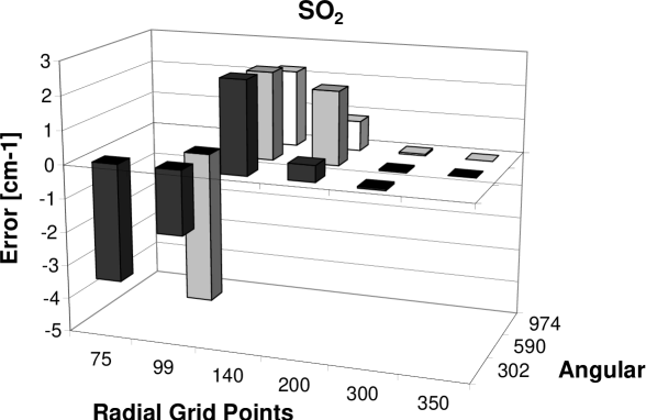
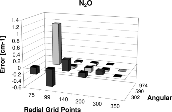
Figure 1: Boese et al

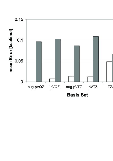
Figure 2: Boese et al

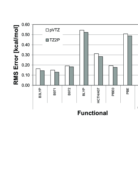
Figure 3: Boese et al

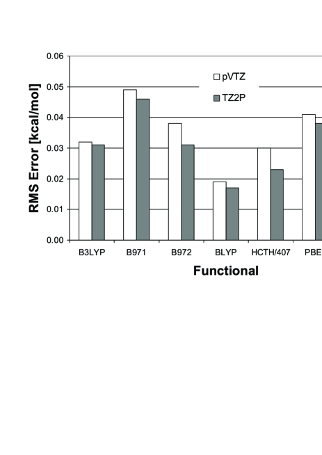
Figure 4: Boese et al

Fig. 1:
Error in the off-diagonal anharmonicity between both stretches. The absolute values for these values at the reference grids are for 172 cm^-1 (H₂O), 12 cm^-1 (SO₂) and 24 cm^-1 (N₂O).

Fig. 2:
Basis set error, together with overall mean error, for the C₂H₄, H₂O, SO₂ and N₂O molecules using different basis sets. The white bars show basis set truncation error relative to aug-cc-pVQZ, while the grey bars show the error compared to the reference values (large basis set CCSD(T), see references).

Fig. 3:
RMS errors of several functionals for the anharmonic ZPVE, compared to to scaled and unscaled harmonic B3LYP values.

Fig. 4:
RMS errors of several functionals for the anharmonic ZPVE, combining CCSD(T) harmonic frequencies and DFT anharmonic corrections.

Table 1: B97-1/TZ2P fundamental frequencies of CH₂NH using different numerical differentiation step sizes. All step sizes are in multiples of 0.01 a.u. unless indicated otherwise.

Method	Uniform (1)			(2)	(3)	(4)	(5)	Richardson extrap.
Mode	2	0.025Å	12	0.025Å		6	4	8/10/12/14	10/12/14
1	3279	3281	3252	3280	3275	3283	3283	3283	3284
2	2996	2996	2987	2995	2995	2995	2997	2997	2997
3	2868	2868	2860	2868	2868	2878	2869	2870	2870
4	1670	1672	1671	1672	1673	1672	1672	1672	1672
5	1458	1460	1461	1460	1462	1460	1460	1460	1460
6	1323	1335	1339	1336	1339	1338	1336	1335	1336
7	1091	1131	1140	1137	1141	1138	1135	1132	1135
8	1045	1073	1079	1077	1081	1079	1076	1074	1076
9	1058	1058	1060	1058	1064	1058	1058	1057	1058

(1) Uniform ‘one size fits all’ step size.

(2) Step size proportional to reduced mass of normal mode, eq. (4)

(3) Step size chosen such that harmonic energy change will amount to 1 millihartree for that mode.

(4) Using eq. (5).

(5) Using eq. (6).

Table 2: Errors (cm^-1) in harmonic frequencies, fundamental frequencies, and anharmonic corrections for several exchange-correlation functionals and basis sets.

Property		Harmonic Frequency		Fundamental Frequency		Correction
Method	Basis set	mean	RMS	mean	RMS	mean	RMS
B3LYP	TZ2P	-4	35	-2	35	-2.4	7.7
	cc-pVTZ	-6	40	-4	39	-1.5	6.1
B97-1	TZ2P	-6	32	-3	32	-3.7	10.5
	cc-pVTZ	-7	37	-3	35	-2.8	8.1
B97-2	TZ2P	8	33	11	38	-2.4	6.7
	cc-pVTZ	8	36	11	39	-2.9	7.8
BLYP	TZ2P	-56	109	-56	108	-0.3	6.2
	cc-pVTZ	-57	109	-57	110	0.1	5.6
HCTH/407	TZ2P	-25	55	-24	56	-1.2	6.8
	cc-pVTZ	-27	58	-25	59	-1.4	6.6
PBE0	TZ2P	7	35	11	40	-3.6	9.3
	cc-pVTZ	7	40	9	43	-2.9	8.2
PBE	TZ2P	-51	93	-49	92	-2.3	9.3
	cc-pVTZ	-52	93	-49	93	-1.6	7.0
scaled B3LYP	cc-pVTZ			24	61	-30	68

Table 3: Errors (cm^-1) for equilibrium and vibrational ground state rotational constants (and difference between them) for several exchange-correlation functionals and basis sets. For the TZ2P basis set, the CH₂ molecule has been excluded in the evaluation. In case of the total values of the rotational constants, all values have been reported in %, with the RMS error corresponding to the RMS error of all the individual % errors.

Property		$B_{e}$ (%)		$B_{0}$ (%)		Correction
Method	Basis set	mean	RMS	mean	RMS	mean	RMS
B3LYP	TZ2P	-0.18	1.05	0.14	1.12	0.015	0.047
	cc-pVTZ	-0.31	1.01	-0.16	1.10	0.008	0.037
B97-1	TZ2P	-0.42	1.01	-0.19	1.03	0.012	0.043
	cc-pVTZ	-0.52	1.11	-0.33	1.22	0.009	0.037
B97-2	TZ2P	0.34	0.92	0.61	1.15	0.015	0.047
	cc-pVTZ	0.34	0.94	0.54	1.13	0.010	0.038
BLYP	TZ2P	-2.28	2.77	-2.19	2.81	0.014	0.051
	cc-pVTZ	-2.30	2.79	-2.31	2.86	-0.002	0.034
HCTH/407	TZ2P	-0.61	1.25	-0.50	1.30	0.005	0.040
	cc-pVTZ	-0.62	1.39	-0.50	1.39	0.005	0.029
PBE0	TZ2P	0.25	0.90	0.59	1.19	0.018	0.051
	cc-pVTZ	0.25	0.95	0.39	1.11	0.010	0.041
PBE	TZ2P	-2.01	2.32	-1.84	2.28	0.018	0.057
	cc-pVTZ	-2.02	2.42	-1.87	2.40	0.005	0.028

Table 4: RMS errors for thermodynamic functions at several temperatures using DFT anharmonic force fields

Property		Heat capacity			Enthalpy function			Entropy
		$C_{p}$ [J/K.mol]			$H-H_{0}$ [kJ/mol]			$S$ [J/K.mol]
Functional	Basis set	298.15	600	2000	298.15	600	2000	298.15	600	2000
B3LYP	TZ2P	0.57	0.42	0.92	0.08	0.23	0.85	0.53	0.83	1.23
	cc-pVTZ	0.61	0.40	0.67	0.09	0.23	0.64	0.95	1.10	1.33
B97-1	TZ2P	0.60	0.41	0.56	0.09	0.24	0.71	0.52	0.86	1.20
	cc-pVTZ	0.64	0.41	0.69	0.10	0.24	0.70	0.54	0.84	1.17
B97-2	TZ2P	0.47	0.45	0.67	0.06	0.24	0.78	0.44	0.82	1.25
	cc-pVTZ	0.54	0.46	0.78	0.08	0.25	0.81	0.46	0.87	1.30
BLYP	TZ2P	0.93	0.96	1.10	0.14	0.43	1.48	1.08	1.69	2.51
	cc-pVTZ	0.91	0.89	1.13	0.15	0.39	1.42	1.05	1.57	2.34
HCTH/407	TZ2P	0.65	0.66	0.66	0.10	0.30	1.00	0.63	1.08	1.65
	cc-pVTZ	0.68	0.65	0.99	0.10	0.29	0.93	0.64	1.02	1.53
PBE0	TZ2P	0.47	0.44	1.02	0.07	0.20	1.00	0.44	0.71	1.30
	cc-pVTZ	0.55	0.45	0.76	0.08	0.22	0.78	0.47	0.76	1.21
PBE	TZ2P	0.90	0.93	1.03	0.14	0.41	1.28	0.94	1.52	2.22
	cc-pVTZ	0.94	0.91	1.12	0.14	0.40	1.27	0.96	1.47	2.15

Table 5: RMS errors for thermodynamic functions at several temperatures using DFT and the RRHO approximation with equilibrium geometries and harmonic frequencies

Property		Heat capacity			Enthalpy function			Entropy
		$C_{p}$ [J/K.mol]			$H-H_{0}$ [kJ/mol]			$S$ [J/K.mol]
Functional	Basis set	298.15	600	2000	298.15	600	2000	298.15	600	2000
B3LYP	TZ2P	0.53	0.78	2.84	0.07	0.25	2.58	0.46	0.85	2.45
	cc-pVTZ	0.54	0.77	2.82	0.07	0.25	2.55	0.88	1.14	2.57
B97-1	TZ2P	0.44	0.71	2.72	0.06	0.21	2.49	0.40	0.72	2.26
	cc-pVTZ	0.46	0.71	2.82	0.06	0.22	2.50	0.42	0.76	2.30
B97-2	TZ2P	0.56	0.83	2.91	0.07	0.24	2.72	0.45	0.81	2.60
	cc-pVTZ	0.60	0.84	2.89	0.08	0.26	2.70	0.49	0.88	2.62
BLYP	TZ2P	0.73	0.54	2.60	0.12	0.31	1.81	0.93	1.37	1.82
	cc-pVTZ	0.66	0.46	2.59	0.12	0.28	1.77	0.88	1.26	1.70
HCTH/407	TZ2P	0.47	0.43	2.62	0.08	0.20	2.04	0.53	0.82	1.72
	cc-pVTZ	0.49	0.48	2.70	0.08	0.15	2.07	0.54	0.55	1.83
PBE0	TZ2P	0.59	0.84	2.90	0.08	0.31	2.71	0.48	1.13	2.64
	cc-pVTZ	0.63	0.89	2.88	0.08	0.37	2.68	0.52	1.43	2.67
PBE	TZ2P	0.61	0.44	2.61	0.11	0.26	1.76	0.79	1.13	1.59
	cc-pVTZ	0.60	0.46	2.58	0.11	0.26	1.72	0.78	1.15	1.55
CCSD(T)		0.28	0.75	3.01	0.03	0.18	2.74	0.26	0.57	2.50

Table 6: RMS errors for thermodynamic functions at several temperatures using DFT and the RRHO approximation with zero-point average geometries and fundamental frequencies

Property		Heat capacity			Enthalpy function			Entropy
		$C_{p}$ [J/K.mol]			$H-H_{0}$ [kJ/mol]			$S$ [J/K.mol]
Functional	Basis set	298.15	600	2000	298.15	600	2000	298.15	600	2000
B3LYP	TZ2P	0.57	0.44	2.44	0.08	0.22	1.78	0.53	0.85	1.60
	cc-pVTZ	0.60	0.45	2.45	0.09	0.23	1.80	0.95	1.14	1.80
B97-1	TZ2P	0.59	0.37	2.35	0.09	0.22	1.66	0.52	0.72	1.53
	cc-pVTZ	0.63	0.45	2.45	0.10	0.23	1.79	0.54	0.76	1.65
B97-2	TZ2P	0.46	0.50	2.50	0.06	0.23	1.94	0.43	0.81	1.82
	cc-pVTZ	0.54	0.54	2.52	0.08	0.25	1.98	0.46	0.88	1.93
BLYP	TZ2P	0.90	0.80	2.19	0.14	0.39	1.16	1.06	1.37	1.57
	cc-pVTZ	0.89	0.76	2.22	0.14	0.37	1.21	1.04	1.26	1.66
HCTH/407	TZ2P	0.62	0.48	2.22	0.09	0.26	1.19	0.62	0.82	1.12
	cc-pVTZ	0.67	0.59	2.33	0.10	0.28	1.42	0.63	0.55	1.35
PBE0	TZ2P	0.46	0.49	2.50	0.07	0.20	1.92	0.43	1.13	1.75
	cc-pVTZ	0.55	0.53	2.51	0.08	0.22	1.93	0.47	1.43	1.82
PBE	TZ2P	0.49	0.82	2.19	0.06	0.39	1.21	0.93	1.13	1.57
	cc-pVTZ	0.93	0.82	2.21	0.14	0.38	1.26	0.95	1.15	1.66
CCSD(T)		0.07	0.29	2.49	0.00	0.06	1.78	0.03	0.14	1.33

Table 7: RMS errors for thermodynamic functions at several temperatures using DFT anharmonic force fields combined with large basis set CCSD(T) geometries and harmonic frequencies

Property		Heat capacity			Enthalpy function			Entropy
		$C_{p}$ [J/K.mol]			$H-H_{0}$ [kJ/mol]			$S$ [J/K.mol]
Functional	Basis set	298.15	600	2000	298.15	600	2000	298.15	600	2000
B3LYP	TZ2P	0.17	0.29	0.90	0.03	0.08	1.05	0.18	0.25	0.90
	cc-pVTZ	0.18	0.26	0.81	0.03	0.08	0.94	0.19	0.24	0.81
B97-1	TZ2P	0.30	0.30	0.93	0.05	0.12	0.99	0.25	0.40	0.93
	cc-pVTZ	0.31	0.29	0.93	0.05	0.12	0.98	0.27	0.39	0.93
B97-2	TZ2P	0.09	0.30	0.93	0.01	0.12	0.99	0.14	0.39	0.93
	cc-pVTZ	0.09	0.30	0.96	0.01	0.12	1.01	0.14	0.39	0.96
BLYP	TZ2P	0.11	0.31	0.87	0.01	0.07	1.02	0.16	0.22	0.87
	cc-pVTZ	0.10	0.28	0.86	0.01	0.07	1.04	0.13	0.16	0.86
HCTH/407	TZ2P	0.18	0.31	0.99	0.03	0.09	1.12	0.16	0.27	0.99
	cc-pVTZ	0.19	0.30	0.93	0.03	0.09	1.06	0.19	0.26	0.93
PBE0	TZ2P	0.10	0.27	0.81	0.01	0.06	0.97	0.15	0.18	0.81
	cc-pVTZ	0.10	0.24	0.74	0.01	0.06	0.89	0.16	0.16	0.74
PBE	TZ2P	0.47	0.36	1.08	0.07	0.18	1.02	0.35	0.59	1.08
	cc-pVTZ	0.50	0.35	1.05	0.07	0.18	0.98	0.37	0.59	1.05

References

- (1) S. Dressler and W. Thiel. Chem. Phys. Lett. 273, 71 (1997).
- (2) P. Hassanzedeh and K. K. Irikura, J. Comp. Chem. 19, 1315 (1998).
- (3) M. O. Sinnokrot and C. D. Sherrill, J. Chem. Phys. 115, 2439 (2001).
- (4) M. Rosenstock, P. Rosmus, E. A. Reinsch, O. Treutler, S. Carter, and N. C. Handy, Mol. Phys. 93, 853 (1998).
- (5) A. Miani, E. Cane, P. Palmieri, A. Trombetti, and N. C. Handy, J. Chem. Phys. 112, 248 (2000).
- (6) I. Baraille, C. Larrieau, A. Dargelos, and M. Chaillet, Chem. Phys. 271, 91 (2001).
- (7) R. Burcl, N. C. Handy, and S. Carter,Spectrochim. Acta A 59, 1881 (2003).
- (8) A. Caligiana, V. Aquilanti, R. Burcl, N. C. Handy, and D. P. Tew, Chem. Phys. Lett. 369, 335 (2003).
- (9) J. Neugebauer and B. A. Hess, J. Chem. Phys. 118, 7215 (2003).
- (10) A. D. Becke, J. Chem. Phys. 98 5648 (1993).
- (11) J. P. Perdew, Phys. Rev. B. 33 8822 (1986).
- (12) V. Barone, J. Chem. Phys. 120, 3059 (2004).
- (13) A. D. Boese and Jan M.L. Martin, J. Phys. Chem. A 108, 3085 (2004).
- (14) V. Barone, J. Phys. Chem. A 108, 4146 (2004).
- (15) S. Parthiban and J. M. L. Martin, J. Chem. Phys. 115, 2051 (2001)
- (16) J. M. L. Martin and G. De Oliveira, J. Chem. Phys. 111, 1843 (1999).
- (17) A. D. Boese, M. Oren, O. Atasoylu, J. M. L. Martin, M. Kallay and J. Gauss, J. Chem. Phys. 120, 4129 (2004).
- (18) For a review see W. Klopper, in R12 methods, Gaussian geminals. in Modern Methods and Algorithms of Quantum Chemistry, 2nd Edition, Ed. J. Grotendorst (John von Neumann Institute for Computing, Jülich, Germany, 2000, pp. 181-229); available online at http://www.fz-juelich.de/nic-series/Volume3/klopper.pdf.
- (19) J. M. L. Martin, J. P. François, and R. Gijbels, J. Chem. Phys. 96, 7633 (1992); J. M. L. Martin, CCSD(T)/PVQZ calculations
- (20) J. Demaison, L. Margules, J. M. L. Martin, and J. E. Boggs, Phys. Chem. Chem. Phys. 4, 3282 (2002).
- (21) I. M. Mills, in: Molecular Spectroscopy: Modern Research, eds. K. Narahari Rao, C. W. Mathews, Vol. 1, Academic Press, New York 1972, pp. 115-140.
- (22) D. A. Clabo Jr., W. D. Allen, R. B. Remington, Y. Yamaguchi, and H. F. Schaefer III, Chem. Phys. 123, 187 (1988).
- (23) W. D. Allen, Y. Yamaguchi, A. G. Csaszar, D. A. Clabo, R. B. Remington, and H. F. Schaefer III, Chem. Phys. 145, 427 (1990).
- (24) W. Schneider and W. Thiel, Chem. Phys. Lett. 157, 367 (1989).
- (25) A. R. Hoy, I. M. Mills, and G. Strey, Mol. Phys. 24, 1265 (1972).
- (26) J. M. L. Martin and S. Parthiban, in: Quantum Mechanical Prediction of Thermochemical Data, eds. J. Cioslowski, Kluwer Academic Publishers, Dordrecht, 2001, Chapter 2, pp. 47.
- (27) N. J. Wright and R. B. Gerber, J. Chem. Phys. 112, 2598 (2000).
- (28) N. J. Wright, R. B. Gerber, and D. J. Tozer, Chem. Phys. Lett. 324, 206 (2000).
- (29) G. M. Chaban and R. B. Gerber, J. Chem. Phys. 115, 1340 (2001).
- (30) G. M. Chaban and R. B. Gerber, Spectrochim Acta A 58, 887 (2002).
- (31) K. Yagi, K. Hirao, T. Taketsugu, M. W. Schmidt, and M. S. Gordon, J. Chem. Phys. 121, 1383 (2004).
- (32) O. Christiansen, J. Chem. Phys. 120, 2140 and 2149 (2004)
- (33) M.J. Frisch, G.W. Trucks, H.B. Schlegel, G.E. Scuseria, M.A. Robb, J.R. Cheeseman, V.G. Zakrzewski, J.A. Montgomery Jr., R. E. Stratmann, J. C. Burant, S. Dapprich, J. M. Millam, A.D. Daniels, K.N. Kudin, M.C. Strain, O. Farkas, J. Tomasi, V. Barone, M. Cossi, R. Cammi, B. Mennucci, C. Pomelli, C. Adamo, S. Clifford, J. Ochterski, G.A. Petersson, P.Y. Ayala, Q. Cui, K. Morokuma, D.K. Malick, A.D. Rabuckm, K. Raghavachari, J.B. Foresman, J. Cioslowski, J.V. Ortiz, A.G. Baboul, B.B. Stefanov, G. Liu, A. Liashenko, P. Piskorz, I. Komaromi, R. Gomperts, R.L. Martin, D.J. Fox, T. Keith, M.A. Al-Laham, C.Y. Peng, A. Nanayakkara, C. Gonzalez, M. Challacombe, P.M.W. Gill, B. Johnson, W. Chen, M.W. Wong, J.L. Andres, C. Gonzalez, M. Head-Gordon, E.S. Replogle, and J.A. Pople, gaussian 98, Revision A.7 (Gaussian, Inc., Pittsburgh, PA, 1998).
- (34) The Cambridge Analytic Derivatives Package (Cadpac), Issue 6.5, Cambridge, 1998 Developed by R. D. Amos with contributions from I. L. Alberts, J. S. Andrews, S. M. Colwell, N. C. Handy, D. Jayatikala, P.J. Knowles, R. Kobayashi,K. E. Laidig, G. Laming, A. M. Lee, P. E. Maslen, C. W. Murray, P. Palmieri, J. E. Rice, E. D. Simandiras, A. J. Stone, M.-D. Su, and D. J. Tozer.
- (35) J. F. Gaw, A. Willets, W. H. Green, and N. C. Handy, in: J. M. Bowman (Ed.), Advances in Molecular Vibration and Collision Dynamics, JAI Press, Greenwich, CT, 1990.
- (36) J. M. L. Martin, “POLYAD: a vibrational perturbation theory program including arbitrary resonance matrices” (Weizmann Institute of Science, Reḥovot, 1997).
- (37) B. J. McBride and S. Gordon, PAC99, Properties and Coefficients code, NASA Reference Publication RP-1271, NASA Lewis/Glenn Research Center, Cleveland, Ohio, 1992.
- (38) J. M. L. Martin, T. J. Lee, and P. R. Taylor, J. Chem. Phys. 108, 676 (1998).
- (39) J. M. L. Martin, T. J. Lee, P. R. Taylor, and J. P. François, J. Chem. Phys. 103, 2589 (1995); J. M. L. Martin and P. R. Taylor, Chem. Phys. Lett. 248, 336 (1996).
- (40) G. de Oliveira, J. M. L. Martin, I. K. C. Silwal, and J. F. Liebman, J. Comp. Chem. 22, 1297 (2001).
- (41) J. M. L. Martin, CCSD(T)/A’VQZ calculations.
- (42) T. J. Lee, J. M. L. Martin, and P. R. Taylor, J. Chem. Phys. 102, 254 (1995).
- (43) J. M. L. Martin, T. J. Lee, and P. R. Taylor, J. Mol. Spect. 160, 105 (1993); J. M. L. Martin, CCSD(T)/PVQZ calculations.
- (44) J. M. L. Martin, CCSD(T)/PVQZ calculations.
- (45) J. M. L. Martin, J. P. François, and R. Gijbels, J. Mol. Spectr. 169, 445 (1995).
- (46) J. M. L. Martin and P. R. Taylor, Chem. Phys. Lett. 205, 535 (1993).
- (47) J. M. L. Martin, J. P. François, and R. Gijbels, J. Chem. Phys. 97, 3530 (1992).
- (48) D. Wang, Q. Shi, and Q.-S. Zhu, J. Chem. Phys. 112, 9624 (2000).
- (49) X.-G. Wang, E. L. Sibert III, and J. M. L. Martin, J. Chem. Phys. 112, 1353 (2000).
- (50) J. M. L. Martin, K. K. Baldridge, and T. J. Lee, Mol. Phys. 97, 945 (1999).
- (51) J. M. L. Martin, J. Chem. Phys. 108, 2791 (1998).
- (52) A. D. Boese and N. C. Handy, J. Chem. Phys. 114 5497 (2001).
- (53) C. W. Murray, N. C. Handy, and G. J. Laming, Mol. Phys 78, 997 (1993)
- (54) V. I. Lebedev, Zh. Vychisl. Mat. Mat. Fiz. 15, 48 (1975); V. I. Lebedev, Zh. Vychisl. Mat. Mat. Fiz. 16, 293 (1976); V. I. Lebedev, Sibirsk. Mat. Zh. 18, 132 (1977); V. I. Lebedev and A. L. Skorokhodov, Russian Acad. Sci. Dokl. Math. 45, 587 (1992)
- (55) R. E. Stratmann, G. E. Scuseria, and M. J. Frisch, Chem. Phys. Lett. 257, 213 (1996)
- (56) T. H. Dunning, J. Chem. Phys. 90, 1007 (1989); R. A. Kendall, T. H. Dunning, and R. J. Harrison, J. Chem. Phys. 96, 6796 (1992).
- (57) A. K. Wilson, K. A. Peterson, and T. H. Dunning Jr., J. Chem. Phys. 114, 9244 (2001).
- (58) T. H. Dunning, J. Chem. Phys. 55, 716 (1971).
- (59) T. H. Dunning Jr. and P. J. Hay, in: Modern Theoretical Chemistry, ed. H. F. Schaefer III, Plenum, New York (1976), vol.3, 1.
- (60) F. A. Hamprecht, A. J. Cohen, D. J. Tozer and N. C. Handy, J. Chem. Phys. 109, 6264 (1998).
- (61) gaussian 03, Revision B.02, M. J. Frisch, G. W. Trucks, H. B. Schlegel, G. E. Scuseria, M. A. Robb, J. R. Cheeseman, J. A. Montgomery, Jr., T. Vreven, K. N. Kudin, J. C. Burant, J. M. Millam, S. S. Iyengar, J. Tomasi, V. Barone, B. Mennucci, M. Cossi, G. Scalmani, N. Rega, G. A. Petersson, H. Nakatsuji, M. Hada, M. Ehara, K. Toyota, R. Fukuda, J. Hasegawa, M. Ishida, T. Nakajima, Y. Honda, O. Kitao, H. Nakai, M. Klene, X. Li, J. E. Knox, H. P. Hratchian, J. B. Cross, C. Adamo, J. Jaramillo, R. Gomperts, R. E. Stratmann, O. Yazyev, A. J. Austin, R. Cammi, C. Pomelli, J. W. Ochterski, P. Y. Ayala, K. Morokuma, G. A. Voth, P. Salvador, J. J. Dannenberg, V. G. Zakrzewski, S. Dapprich, A. D. Daniels, M. C. Strain, O. Farkas, D. K. Malick, A. D. Rabuck, K. Raghavachari, J. B. Foresman, J. V. Ortiz, Q. Cui, A. G. Baboul, S. Clifford, J. Cioslowski, B. B. Stefanov, G. Liu, A. Liashenko, P. Piskorz, I. Komaromi, R. L. Martin, D. J. Fox, T. Keith, M. A. Al-Laham, C. Y. Peng, A. Nanayakkara, M. Challacombe, P. M. W. Gill, B. Johnson, W. Chen, M. W. Wong, C. Gonzalez, and J. A. Pople, Gaussian, Inc., Pittsburgh PA, 2003.
- (62) see Eq. (13) in http://www.gaussian.com/g_whitepap/vib.htm
- (63) A. Ralston and P. Rabinowitz, A first course in numerical analysis, 2nd ed. (Dover, New York, 2001), Section 4.2.
- (64) A. D. Becke, Phys. Rev. A 38 3098 (1988), C. Lee, W. Yang, R. G. Parr, Phys. Rev. B 37 785 (1988).
- (65) J. P. Perdew, K. Burke, and M. Ernzerhof, Phys. Rev. Lett. 77, 3865 (1996).
- (66) P. J. Wilson, T. J. Bradley, and D. J. Tozer, J. Chem. Phys. 115, 9233 (2001).
- (67) C. Adamo and V. Barone, Chem. Phys. Lett. 298, 113 (1998).
- (68) A. D. Boese, J. M. L. Martin, and N. C. Handy, J. Chem. Phys. 119, 3005 (2003).
- (69) A. D. Boese and J. M. L. Martin, J. Chem. Phys. 121, 3405 (2004).
- (70) A. D. Boese and N.C. Handy, J. Chem. Phys. 116, 9559 (2002).
- (71) Paraphrasing T. S. Eliot’s Murder in a Cathedral: “The last temptation is the greatest treason/To get the right answer for the wrong reason”