Asymmetric polarity reversals, bimodal field distribution, and coherence resonance in a spherically symmetric mean-field dynamo model

Abstract

Using a mean-field dynamo model with a spherically symmetric helical turbulence parameter $\alpha$ which is dynamically quenched and disturbed by additional noise, the basic features of geomagnetic polarity reversals are shown to be generic consequences of the dynamo action in the vicinity of exceptional points of the spectrum. This simple paradigmatic model yields long periods of constant polarity which are interrupted by self-accelerating field decays leading to asymmetric polarity reversals. It shows the recently discovered bimodal field distribution, and it gives a natural explanation of the correlation between polarity persistence time and field strength. In addition, we find typical features of coherence resonance in the dependence of the persistence time on the noise.

The Earth’s magnetic field is known to undergo irregular polarity reversals, with a mean reversal rate that varies from zero in the Permian and Cretaceous supercrons to (4-5) per Myr in the present MERR . Typically, these reversals have an asymmetric (saw-toothed) shape, i.e. the field of one polarity decays slowly and recovers very rapidly with the opposite polarity, possibly to rather high intensities VALET-MEYN-BOGU . A general correlation between the persistence time and the field intensity has also been suspected since long COX-TARDUNO . A recent observation concerns the bimodal distribution of the Earth dipole moment with two peaks at about 4 $\times$ 10²² Am² and at about twice that value HELLER .

The explanation of these phenomena represents a great challenge for dynamo theory and numerics. Remarkably, the last decade has seen three-dimensional numerical simulations of the geodynamo with sudden polarity reversals as one of the most impressive results (cf. GLRO-ANDCO for a recent overview).

Despite the fact that those simulations exhibit many features of the Earth’s magnetic field quite well, and because they do so in parameter regions (in particular for the Ekman and the magnetic Prandtl number) that are far away from the real ones, there is a complimentary tradition to identify the essential ingredients of reversals within the framework of simplified dynamo models. This has been done, e.g., in the tradition of the celebrated Rikitake dynamo model of two coupled disk dynamos RIKI-FRANCK-HIDE . Another approach has been pursued by Hoyng and collaborators HOYNG who studied a prototype nonlinear mean-field dynamo model which is reduced to an equation system for the amplitudes of the non-periodic axisymmetric dipole mode and for one periodic overtone under the influence of stochastic forcing. Interestingly, even this simple model shows sudden reversals and a Poissonian distribution of the polarity persistence time. However, an essential ingredient of this model to account for the correct reversal duration and persistence time is the use of a large turbulent resistivity which is hardly justified, at least not by the recent dynamo experiments RMP .

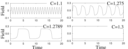
Figure 1: Magnetic field evolution for vanishing noise ($D=0$) and different values of $C$. ”Field” corresponds to $s_{1}(r=0.95)$.

Sarson and Jones SAJO had noticed the importance of the transition from non-oscillatory to oscillatory states for reversals to occur. It is our goal to understand this process in more detail by studying a simple mean-field dynamo model. We focus on the magnetic field dynamics in the vicinity of ”exceptional points” KATO-HEIS of the spectrum of a non-selfadjoint operator. We will show that the main characteristics of Earth magnetic field reversals can be attributed to the square-root character of the spectrum in the vicinity of such exceptional points, where two non-oscillatory eigenmodes coalesce and continue as an oscillatory eigenmode.

Our starting point is the well known induction equation ${\dot{\bm{B}}}={\bm{\nabla}}\times(\alpha{\bm{B}})+(\mu_{0}\sigma)^{-1}\Delta{\bm{B}}$ for a mean-field dynamo with a helical turbulence parameter $\alpha$ KRRA , acting in a fluid with electrical conductivity $\sigma$ within a sphere of radius $R$. The magnetic field has to be divergence-free,${\bm{\nabla}}\cdot{\bm{B}}=0$. Henceforth, we will measure the length in units of $R$, the time in units of $\mu_{0}\sigma R^{2}$, and the parameter $\alpha$ in units of $(\mu_{0}\sigma R)^{-1}$. Note that for the Earth we get a time scale $\mu_{0}\sigma R^{2}\sim 200$ Kyr, giving a free decay time of 20 Kyr for the dipole field.

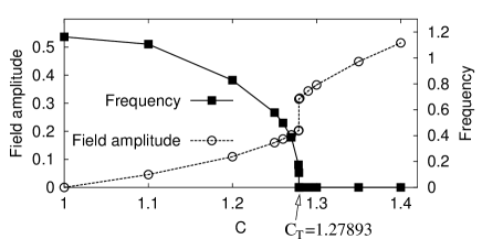
Figure 2: Magnetic field amplitude and frequency for $D=0$ in dependence on $C$. Note the phase transition at $C_{T}=1.27893$.

We decompose ${\bm{B}}$ into a poloidal and a toroidal part, ${\bm{B}}=-\nabla\times({\bm{r}}\times\nabla S)-{\bm{r}}\times\nabla T$. The defining scalars $S$ and $T$ are expanded in spherical harmonics of degree $l$ and order $m$ with the expansion coefficients $s_{l,m}(r,t)$ and $t_{l,m}(r,t)$. In order to allow for very long simulations (to get a good statistics for the persistence time and the field amplitudes), we consider an $\alpha^{2}$ dynamo with a radially symmetric helical turbulence parameter $\alpha$. In OSZI we had shown that such simple $\alpha^{2}$ dynamos can exhibit oscillatory behaviour in case that $\alpha(r)$ changes its sign along the radius, which is not unrealistic for the Earth SOW-RUED . For spherically symmetric and isotropic $\alpha$, the induction equation decouples for each $l$ and $m$ into the following pair of equations:

$$\frac{\partial s_{l}}{\partial t} = \frac{1}{r}\frac{d^{2}}{dr^{2}}(rs_{l})-\frac{l(l+1)}{r^{2}}s_{l}+\alpha(r,t)t_{l}\;,$$ (1)

$$\frac{\partial t_{l}}{\partial t} = \frac{1}{r}\frac{d}{dr}\left(\frac{d}{dr}(rt_{l})-\alpha(r,t)\frac{d}{dr}(rs_{l})\right)$$ (2)

$$-\frac{l(l+1)}{r^{2}}[t_{l}-\alpha(r,t)s_{l}]\;.$$

These equations are independent of the order $m$, hence we have skipped it in the index of $s$ and $t$. The boundary conditions are $\partial s_{l}/\partial r|_{r=1}+{(l+1)}s_{l}(1)=t_{l}(1)=0$.

In the following we restrict ourselves to the dipole field with $l=1$ (the influence of higher multipole fields will be considered elsewhere). At first, we choose a particular radial profile $\alpha(r)$ which can yield an oscillatory behaviour OSZI . Magnetic field saturation is ensured by quenching the parameter $\alpha(r,t)$ with the angular averaged dipole field energy which can be expressed in terms of $s_{1}(r,t)$ and $t_{1}(r,t)$. In addition to that, we perturb the $\alpha$-profile by noisy ”blobs” which are assumed constant within a correlation time $\tau$. In summary, $\alpha(r,t)$ takes the form:

$$\alpha(r,t) = C\frac{-21.5+426.4\;r^{2}-806.7\;r^{3}+392.3\;r^{4}}{1+E\left[\frac{2s_{1}^{2}(r,t)}{r^{2}}+\frac{1}{r^{2}}\left(\frac{\partial(rs_{1}(r,t))}{\partial r}\right)^{2}+t_{1}^{2}(r,t)\right]}$$ (3)

$$+\xi_{1}(t)+\xi_{2}(t)\;r^{2}+\xi_{3}(t)\;r^{3}+\xi_{4}(t)\;r^{4}\;,$$

where the noise correlation is given by $\langle\xi_{i}(t)\xi_{j}(t+t_{1})\rangle=D^{2}(1-|t_{1}|/\tau)\Theta(1-|t_{1}|/\tau)\delta_{ij}$. $C$ is a normalized dynamo number measuring the overcriticality, $D$ is the noise amplitude, and $E$ is a constant measuring the inverse equipartition field energy.

The equation system (1)-(3) is time-stepped using an Adams-Bashforth method with a radial grid spacing of 0.02 and a time step length of 2 $\times$ 10^-5. For the following examples, the correlation time $\tau$ has been set to 0.02, and $E$ has been chosen to be 0.01.

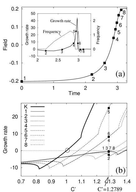
Figure 3: (a) Details of the field evolution for $C=1.2789$ (cf. Fig. 1), with growth rates and frequencies (inset) resulting from the instantaneous, quenched $\alpha$ profiles. (b) Growth rate curves for instantaneous $\alpha$ profiles scaled by $C^{\prime}$. ”K” denotes the kinematic (unquenched) $\alpha$ profile with the (encircled) critical point at $C^{\prime}=1$.

For the noise-free case ($D=0$), we show in Fig. 1 the evolution of the magnetic field for different values of $C$ (hereafter, ”field” stands always for the value of $s_{1}$ at $r=0.95$). At the slightly overcritical value $C=1.1$ we observe a nearly harmonic oscillation with a frequency close to one. With increasing $C$, this frequency decreases, and at the same time the signal becomes saw-toothed (or better: ”shark-fin shaped”) and eventually rectangular. At the critical point $C_{T}=1.27893$ a phase transition to a non-oscillatory dynamo occurs, which can also be identified in the frequencies and field amplitudes shown in Fig. 2.

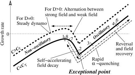
Figure 4: Illustration of the various phases of reversals in the vicinity of an exceptional point of the spectrum. In the noise free case (D=0) oscillatory and steady dynamos can be sharply distinguished. For $D>0$, we get a bimodal behaviour around the maximum of the non-oscillatory branch.

In Fig. 3, we analyze the field evolution for $C=1.2789$ in detail. Figure 3a shows the field during one reversal, together with the growth rate and the frequency that result from the instantaneous, quenched $\alpha$-profile. Eight of these profiles (at the moments 1-8), together with the unquenched profile, are scaled by a factor $C^{\prime}$ yielding the growth rate curves of Fig. 3b. These curves may help us to identify the following phases for a reversal: a slowly starting, but self-accelerating field decay in the non-oscillatory branch (points 1 and 2), followed by the actual polarity reversal in the oscillatory branch (between points 3 and 4), a fast increase of the field (points 4-6) which results in a rapid $\alpha$-quenching. This rapid quenching drives the system back to the point 8 which basically corresponds to the initial point 1, only with the opposite field polarity. A peculiarity of our particular model is the existence of a second exceptional point beyond which the dynamo becomes non-oscillatory again (between points 5 and 6), which is, however, not crucial for the indicated reversal process.

In an attempt to simplify this reversal picture, we consider in Fig. 4 all growth rate curves of Fig. 3b as being collapsed into a single one (for that purpose we neglect their slight shape differences and consider only a shift). By this ”optical trick”, the various phases of reversals can be visualized as a ”move” of the actual growth rate point relative to this collapsed growth rate curve. Figure 4 explains also the phase transition between oscillatory and steady dynamos and the discontinuity of the field amplitude from Fig. 2. The local maximum of the non-oscillatory branch of the growth rate curve is unstable and repels the dynamo in two different directions, depending on whether the growth rate there is negative or positive. If it is negative, the field decays, we get weaker $\alpha$ quenching, and a subsequent reversal. If it is positive, the field increases, we get stronger $\alpha$ quenching, hence the system moves to the left of the maximum.

Figure 5: Time series for $C=1.27$ and $C=1.29$ at $D=0.5$.

What happens now if we switch on the noise? The influence of the noise is quite different for values of $C$ below and above $C_{T}$. For $C>C_{T}$, the noise is the only possibility to trigger a move from left of the local maximum to the right, hence the persistence time will decrease from infinity to some finite value. For $C<C_{T}$, the noise will sometimes push the maximum above the zero growth rate line allowing the system to jump to the left of the maximum where it can stay for a while. Hence, we will get an increase of the persistence time.

For a moderate noise intensity $D=0.5$, we depict in Fig. 5 the time evolution for the values $C=1.27$ and $C=1.29$ which are slightly below and above $C_{T}$, respectively. First of all, a drastic difference between the persistence times is still visible. The duration of a reversal, however, is quite identical for both values of $C$, although its sensible definition is not obvious. With a side view on the real geomagnetic field (for which the dipole component should decay approximately to the strength of the non-dipole components before a reversal can be identified), we tentatively define the reversal duration as the time the field spends between $\pm 1/4$ or $\pm 1/10$ of its mean intensity. In the first case we get a reversal duration of 30 Kyr, in the second case of 12 Kyr, which comes close to the observational facts.

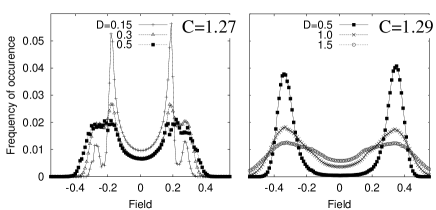
Figure 6: Field histogram for $C=1.27$ and $C=1.29$.

For both values, $C=1.27$ and $C=1.29$, a bimodal behaviour of the dynamo can be observed in the field histograms of Fig. 6. For $C=1.27$ and $D=0.15$, we observe a clear double peak on both polarity sides, centered approximately at $\pm 0.18$ and $\pm 0.27$. Evidently, the dynamo is mostly in the weak field state (right of the maximum, cp. Fig. 4), with some ”excursions” to the strong field state (left of the maximum). With increasing $D$ this double peak is smeared out, leaving a very broad maximum for $D=0.5$. The three histograms for $C=1.29$ show a maximum at the strong field value and (although not a maximum) a pronounced flattening at the weak field value. This means, the dynamo is mostly in the strong field state, with some intermediate stopovers in the weak field state, from where it can start a reversal.

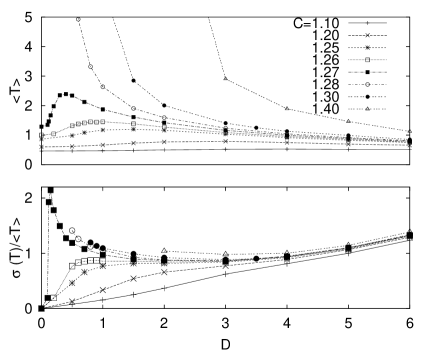
Figure 7: Persistence time $\langle T\rangle$ and its normalized standard deviation $\sigma(T)/\langle T\rangle$ for different $C$ in dependence on $D$. For each point, a minimum of 10⁴ reversals was used.

An overview about the mean persistence time $\langle T\rangle$ and its normalized standard deviation $\sigma(T)/\langle T\rangle$ in dependence on $C$ and $D$ is given in Fig. 7. Note the drastic difference that small values of noise have on the dynamo behaviour for $C<C_{T}$ and $C>C_{T}$. The normalized standard deviation, at least for the curves with $C>1.26$, has a clear minimum around $D=3$ which represents a typical feature of coherence resonance KURTHS . We only note here that recently stochastic resonance models have been discussed with view on a possible triggering of field reversals by the 100 Kyr period of the Earth orbit eccentricity STOCH .

To summarize, our simple spherically symmetric $\alpha^{2}$ dynamo model shows that asymmetric polarity reversals and bimodal field distributions are generic features of the dynamo behaviour in the vicinity of exceptional points. Using only the molecular resistivity of the outer core, we get typical persistence times of the order of 200 Kyr (and larger), and a typical reversal duration of 10-30 Kyr.

We point out that this model is not a physical model of the Earth dynamo, in particular owing to the missing North-South asymmetry of $\alpha$. Nevertheless, we are convinced that the generic features of dynamos in the vicinity of exceptional points as they were illustrated in this paper can also be identified in much more elaborated dynamo models.

References

- (1) R. T. Merrill, M.W. McElhinny, and P.L. McFadden, The Magnetic Field of the Earth, (Academic, San Diego, 1996).
- (2) J.-P. Valet and L. Meynadier, Nature 366, 234 (1993); L. Meynadier et al., Earth Planet. Sci. Lett. 126, 109 (1994); S. W. Bogue and H. A. Paul, Geophys. Res. Lett. 20, 2399 (1993).
- (3) A. Cox, J. Geophys. Res. 73, 3247 (1968); J. A. Tarduno, R. D. Cottrell, and A. V. Smirnov, Science 291, 1779 (2001).
- (4) R. Heller, R. T. Merrill, and P. L. McFadden, Phys. Earth Planet. Inter. 135, 211 (2003).
- (5) G. A. Glatzmaier, Annu. Rev. Earth Planet. Sci. 30, 237 (2002).
- (6) T. Rikitake, Proc. Cambridge Phil. Soc. 54, 89 (1958); F. Plunian, P. Marty, and A. Alemany, Proc. R. Soc. London, Ser. A 454, 1835 (1995).
- (7) P. Hoyng, M. A. J. H. Ossendrijver, and D. Schmidt, Geophys. Astroph. Fluid Dyn. 94, 263 (2001); D. Schmitt, M. A. J. H. Ossendrijver, and P. Hoyng, Phys. Earth Planet. Inter. 125, 119 (2001); P. Hoyng, D. Schmitt, and M. A. J. H. Ossendrijver, Phys. Earth Planet. Inter. 130, 143 (2002).
- (8) A. Gailitis et al., Rev. Mod. Phys. 74, 973 (2002).
- (9) G. R. Sarson and C. A. Jones, Phys. Earth Planet. Inter. 111, 3 (1999).
- (10) T. Kato, Perturbation Theory of Linear Operators, (Springer, Berlin, 1966); W. D. Heiss, Czech. J. Phys. 54, 1091 (2004); U. Günther, F. Stefani, and G. Gerbeth, Czech. J. Phys. 54, 1075 (2004), math-ph/0407015.
- (11) F. Krause and K.-H. Rädler, Mean-field Magnetohydrodynamics and Dynamo Theory, (Akademie-Verlag, Berlin, 1980).
- (12) F. Stefani and G. Gerbeth, Phys. Rev. E 67, 027302 (2003).
- (13) G. Rüdiger and R. Hollerbach, The Magnetic Universe, (Wiley-VCH, Weinheim, 2004), p. 124.
- (14) A. S. Pikovsky and J. Kurths, Phys. Rev. Lett. 78, 775 (1997).
- (15) T. Yamazaki and H. Oda, Science 295, 2435 (2002); G. Consolini and P. De Michelis, Phys. Rev. Lett. 90, 058501 (2003).