Relativistic two-photon bremsstrahlung

Abstract

An approximate approach for the description of the two-photon bremsstrahlung emitted by a relativistic projectile scattered in a spherically-symmetric field is developed. It based on the accurate treatment of the analytical structure of the singularities in relativistic one-photon free-free matrix elements. For the case of a Coulomb field the analytical expressions for the amplitude and cross section of process are presented. Numerical results obtained within the framework of the proposed approach are compared with the available experimental data and with the results of simpler theories.

1 Introduction

In this paper new results from the relativistic theory of two-photon bremsstrahlung (2BrS) of a projectile electron scattered in a spherically-symmetric static field are reported. We formulate the approximation suitable for effective analytical and numerical treatment of a rather complex relativistic free-free two-photon matrix element. The developed formalism is applied to the 2BrS process in a point-Coulomb field. Results of numerical calculation of the 2BrS cross section for several geometries of the emission, incident electron energies and photon frequencies are presented.

The approach, which is described in this paper, based on the use of a so-called ‘delta’-approximation. This method, initially formulated for a non-relativistic 2BrS [1]–[4] and extended later to the case of relativistic collisions [5], is based on the assumption that to a great extent the behaviour of the free-free two-photon amplitude is defined by the contributions of the delta-singular parts of the one-photon matrix elements from which the 2BrS amplitude is constructed.

Transitions of such type are encountered not only in the 2BrS problem but in a number of other physical processes in which the collision of a projectile with a target is accompanied by emission/absorption of photons (see, e.g., reviews [6, 7, 8]). The list of such processes includes, in particular, (a) the bremsstrahlung-type phenomena in an external field (many-photon spontaneous bremsstrahlung, laser-induced bremsstrahlung), (b) various inelastic processes, when the emission/absorption of the photon is accompanied by simultaneous excitation or ionization of the target, (c) Compton scattering from many-electron atoms, (d) many-photon ionization of atoms and ions.

In the case when perturbation theory in photon-projectile (or photon-atom) interaction is used to analyze the above-mentioned processes, the corresponding amplitude ${\cal M}$ can be represented in terms of the compound matrix element which contains the radiative free-free matrix element between the intermediate virtual states and in which the integration over the intermediate momentum is carried out. The general form of such matrix element is

$${\cal M}=\sum_{\mu_{\rm b}}\int{\rm d}{\bf p}_{{\rm b}}\,{\cal R}_{\mu_{\rm b}}({\bf p}_{{\rm b}})\,D^{(\pm\pm)}_{\nu_{\rm b}\nu_{\rm a}}({\bf k},{\bf e})\,.$$ (1)

Here $D^{(\pm\pm)}_{\nu_{\rm b}\nu_{\rm a}}({\bf k},{\bf e})$ stands for the matrix element of the one-photon free-free transition between two relativistic states of a continuous spectrum with momenta ${\bf p}_{{\rm a}}$ and ${\bf p}_{{\rm b}}$ and polarizations $\mu_{\rm a}$ and $\mu_{\rm b}$:

$$D^{(\pm\pm)}_{\nu_{\rm b}\nu_{\rm a}}({\bf k},{\bf e})=\int{\rm d}{\bf r}\,\Psi^{(\pm)\,\dagger}_{\nu_{\rm b}}({\bf r})\,({\bf e}\bm{\alpha})\,\exp{(-{\rm i}{\bf k}{\bf r})}\,\Psi^{(\pm)}_{\nu_{\rm a}}({\bf r})\,.$$ (2)

Here $\Psi^{(\pm)}_{\nu}({\bf r})$ are the bispinor wavefunctions corresponding to the out- (the upper index ‘$+$’) and to the in (‘$-$’) scattering states, the symbol $\dagger$ denotes the hermitian conjugation, $\bm{\alpha}=\gamma^{0}\bm{\gamma}$ where $\gamma^{0}$, $\bm{\gamma}$ are the Dirac matrices. The vectors $\hbar{\bf k}$ and ${\bf e}$ denote the photon momentum and polarization. We choose the gauge in which ${\bf e}{\bf k}=0$. The CGS system is used throughout the paper.

The factor ${\cal R}_{\mu_{\rm b}}({\bf p}_{{\rm b}})$ represents the contribution of all the remaining processes related to the collision. In particular, in the case of 2BrS process, ${\cal R}_{\mu_{\rm b}}({\bf p}_{{\rm b}})$ contains another free-free matrix element (see general expression (6) for the 2BrS amplitude).

Relation (2) defines four matrix elements the type of which depends on the asymptotic behaviour of the wavefunctions of the initial and final states. In the vicinity of the points defined by the relations

$${\bf p}_{{\rm a}}-{\bf p}_{{\rm b}}-\hbar{\bf k}=0\,,\ \quad p_{{\rm a}}-\left|{\bf p}_{{\rm b}}+\hbar{\bf k}\right|=0\,,\ \quad|{\bf p}_{{\rm a}}-\hbar{\bf k}|-p_{{\rm b}}=0\ ,$$ (3)

the matrix elements ${D^{(\pm\pm)}_{\nu_{\rm b}\nu_{\rm a}}({\bf k},{\bf e})}$ contain the singular terms of the two essentially different types [5]. Firstly, there are well known pole-like singularities which are responsible, in particular, for the infrared divergency of the one-photon bremsstrahlung amplitude (see, e.g., [9, 10, 11]. In this case both momenta, ${\bf p}_{{\rm a}}$ and ${\bf p}_{{\rm b}}$, lie on the mass surface, so that the exact equalities (3) are inconsistent with the energy conservation law, which can be written as $\varepsilon_{\rm a}=\varepsilon_{\rm b}+\hbar\,\omega$ (here $\varepsilon_{\rm a,b}$ are the energies of the projectile in the states ’a’ and ’b’, $\hbar\,\omega$ is the photon energy). Hence, in this case the equality signs must be understood as the limits $\to 0$.

The singularities of the second type (we call them ‘delta’ singularities) contain terms proportional to the delta-functions $\delta({\bf p}_{{\rm a}}-{\bf p}_{{\rm b}}-\hbar{\bf k})$, $\delta(p_{{\rm a}}-|{\bf p}_{{\rm b}}+\hbar{\bf k}|)$ and $\delta(|{\bf p}_{{\rm a}}-\hbar{\bf k}|-p_{{\rm b}})$ (note, that the first of these is the three-dimensional $\delta$-function, whereas the two others are one-dimensional). In the compound matrix elements (1) one of the states ‘a’ or ‘b’ (or both, if the process includes the emission of two and more photons, or if the photon emission occurs between two virtual states) describes the off-mass surface particle. Therefore, the ‘delta’ terms add a non-zero contribution to the amplitude (1).

The approach for the approximate treatment (the ‘delta’-approximation) of the compound matrix elements of the type (1) is based on the assumption that to a great extent the behaviour of ${\cal M}$ is defined by the contributions of the delta-singular parts of the one-photon free-free matrix elements $D^{(\pm\pm)}_{\nu_{\rm b}\nu_{\rm a}}({\bf k},{\bf e})$. Initially [1, 2, 3] it was formulated in connection with the problem of two-photon dipole free-free transitions of a non-relativistic projectile moving in an external field of atomic target. In the cited papers as well as in [4, 12] it was demonstrated that over wide regions of the incident electron energies and the photon frequencies the approximate approach produces nearly the same results as the rigorous treatment for both dipole [13, 14, 15, 16] and non-dipole [4, 17] photons.

Within the framework of the non-relativistic dipole-photon approximation it was demonstrated that for the correct evaluation of (1) it is necessary to take into account all singular terms of the free-free matrix elements, and in many cases the contribution of the delta-terms to the integral on the right-hand side is highly noticeable, if not dominant. Such an analysis has been carried out in connection with many-photon ionization (detachment) [18, 19, 20, 21], the single-photon bremsstrahlung process with simultaneous ionization of the target [22], the process of two-photon bremsstrahlung [23, 24], and the process of spontaneous bremsstrahlung in presence of a laser field [25]. In non-relativistic non-dipole approximation the analogous treatment has been applied so far to the free-free compound matrix element which characterizes the amplitude of two-photon bremsstrahlung [3, 4].

A detailed review of the achievements of the non-relativistic theory of 2BrS can be found in [4, 5]. Here we just mention the main results obtained in this field.

Theoretical activity was stimulated by a series of experiments [26, 27, 29, 30, 31, 32, 28, 33] in which the data on the 2BrS cross section and angular distribution were obtained for relatively high energies of the incident electron and emitted photon (up to 70 keV). Apart from the early work of Smirnov [34], where the 2BrS process was treated in terms of the relativistic first Born approximation (see also [35]), theoretical investigations were based on second order non-relativistic perturbation theory. Within the framework of this approximation the exact analytical formulae were obtained for the compound free-free matrix element in the Coulomb field. It was done in the dipole-photon case [36, 15, 13, 14, 23] and with the retardation effects included [4, 17] as well. For neutral atomic targets the calculations of the 2BrS spectrum were performed within the frame of the potential (‘ordinary’) bremsstrahlung model [37, 1, 12] as well as with the 2BrS emission due to the ‘polarizational’ bremsstrahlung mechanism taken into account [38, 39, 40].

In connection with the experiments [29, 30, 31, 32], where the 2BrS process was studied for 70 keV electrons scattered by various many-electron atoms, it was noted in several publications [1, 3, 4, 16, 17, 41] that the role of the retardation effects in the 2BrS process is much higher than in the conventional one-photon bremsstrahlung. In these papers it was also demonstrated that that for the energies of the electron and the photons within the tens of keV range (i.e. as in the cited experiments) it is the retardation and relativistic effects which are mostly important for the formation of the 2BrS spectrum rather than the effect of screening due to atomic electrons. The inclusion of the latter effect in the calculation scheme mofifies the result on the level of several per cent (see, e.g., [1]) whereas the account for the radiation retardation increases the 2BrS cross section by the order of magnitude [4, 17]. Therefore, to obtain a reliable theoretical result one has not only go beyond the frame of the non-relativistic dipole-photon approximation but to consider the fully relativistic treatment of the problem.

The relativistic treatment of the compound many-photon transitions is much more complicated than its non-relativistic analogue from both analytical and computational viewpoints [42, 43, 44, 45, 46, 47, 48, 49, 50, 51, 52, 53]. In the cited papers the theory and the numerical results for various processes described by the two-photon bound-bound and bound-free transitions are presented. In contrast, the exact relativistic treatment of the free-free two-photon transitions has not been suggested so far. Till recently all theoretical considerations did not go beyond the framework of the plane wave first Born approximation [34, 35] and the soft-photon limit [54]. In the recent paper [5] the relativistic formalism of ‘delta’-approximation for treatment of many-photon free-free transitions was developed. Its application was illustrated by the evaluation of the delta-amplitude of 2BrS process. Excluding the papers [34, 35, 54] there were no numerical results of relativistic calculations of 2BrS cross sections.

In order to fill this gap we extend the approximate treatment of the relativistic 2BrS developed in [5] to the case of the point Coulomb field, $-Ze/r$, and perform a numerical analysis of the role of retardation and relativistic effects in the formation of spectral and angular distributions of 2BrS for the conditions of the experiments [29, 30, 31, 32]. This is done within the framework of the ‘delta’-approximation, described in more detail in [5] and in section 2 below. Because of the absence of the closed analytic expression for the relativistic scattering states wavefunctions we used the Furry-Sommerfeld-Maue (FSM) wavefunctions (e.g. [9]). The applicability of FSM approximation in view of available experimental data is discussed in section 2.3.

In spite of the fact that the validity of the ‘delta’-approximation has not been formally proved there is a number of indirect confirmations of the applicability of this approach. In particular it was demonstrated (both in the non-relativistic [3] and relativistic [5] cases) that the general expression for the ’delta’-amplitude of the 2BrS process correctly reproduces the important limiting cases: the plane-wave first Born approximation and the soft-photon approximation. Also the ‘delta’-approximation, being applied for the description of a number of mentioned above processes, yields reasonable numerical results against the results of the exact calculations. In the dipole-photon regime it was done for the two-photon bremsstrahlung [1, 2, 12, 24], two- and three-photon detachment of electrons from negative ions [55]. Beyond the dipole-photon approximation the comparison was carried out for the 2BrS process of a non-relativistic electron [3, 4].

This approach, although being approximate, allows us to evaluate effectively the principal parts of the free-free two-photon matrix element in the relativistic domain with much less analytical and computational efforts. The method can be generalized to embrace the $n$-photon ($n>2$) radiative free-free transitions.

The formalism is described in section 2. In section 3 we present the results of numerical calculations and carry out the comparison with available experimental data and the results of simpler theories.

2 Formalism

2.1 2BrS amplitude and cross section: general formulae

Figure 1: Diagrammatical representation of the 2BrS process. The solid lines correspond to the relativistic projectile moving in an external field of the target (the Furry picture, e.g. [9]). The transition from the initial state ‘1’ into the final state ‘2’ via the intermediate (virtual) state ‘n’ is accompanied by the emission of two photons $\gamma_{1,2}$ (the dashed lines).

The 2BrS process during the potential scattering of an electron (the charge is labeled as $e$ and the mass as $m_{\rm p}$) is a transition of the projectile from the initial state $\nu_{1}=({\bf p}_{1},\mu_{1})$ to the final state $\nu_{2}=({\bf p}_{2},\mu_{2})$ accompanied by the emission of two photons. Each of the photons ($j=1,2$) is characterized by the energy, $\hbar\omega_{j}$, momentum $\hbar{\bf k}_{j}$ and the polarizational vector ${\bf e}_{j}$. The energies of all particles satisfy the energy conservation law

$$\varepsilon_{1}=\varepsilon_{2}+\hbar\omega_{1}+\hbar\omega_{2}\ .$$ (4)

where $\varepsilon_{1,2}=\sqrt{p_{1,2}^{2}c^{2}+m_{\rm p}^{2}c^{4}}$ are the particle energies in the initial and the final states.

The four-fold cross section differential with respect to $\omega_{1,2}$ and to the solid angles of the photons emission $\Omega_{1,2}$ is given by

$${{\rm d}^{4}\sigma\over{\rm d}\omega_{1}\,{\rm d}\omega_{2}\,{\rm d}\Omega_{1}\,{\rm d}\Omega_{2}}={\alpha^{2}\over 2}\,{\varepsilon_{1}\varepsilon_{2}\over c^{4}}\,{p_{2}\over p_{1}}\,{\omega_{1}\,\omega_{2}\over(2\pi)^{6}}\,\sum_{\lambda_{1},\lambda_{2}}\sum_{\mu_{1},\mu_{2}}\int_{(4\pi)}{\rm d}\Omega_{{\bf p}_{2}}\,\left|{\cal M}\right|^{2}\,.$$ (5)

Here $\alpha$ is the fine structure constant, the integration is performed over the solid angle of the scattered particle, the summations are carried out over the polarizations of the photons ($\lambda_{1,2}$) and of the projectile ($\mu_{1,2}$).

The total amplitude of the process, ${\cal M}$, is described by two Feynman diagrams as presented in figure 1. Each diagram corresponds to the compound matrix element of the two-photon transition from the initial state ‘1’ via the intermediate (virtual) state ‘$n$’ to the final state ‘2’:

$${\cal M}={\cal M}_{[12]}+{\cal M}_{[21]}\,,\quad{\cal M}_{[12]}=\sum_{n}{\langle{\bf p}_{2}\mu_{2}|{\bf e}_{2}\bm{\gamma}\,{\rm e}^{-{\rm i}{\bf k}_{2}{\bf r}}|n\rangle\langle n|{\bf e}_{1}\bm{\gamma}\,{\rm e}^{-{\rm i}{\bf k}_{1}{\bf r}}|{\bf p}_{1}\mu_{1}\rangle\over\varepsilon_{n}+\hbar\omega_{1}-\varepsilon_{1}-{\rm i}0}\,.\quad$$ (6)

Here $\langle{\bf p}_{2}\mu_{2}|\equiv\Psi_{{\bf p}_{2}\mu_{2}}^{(-)\,\dagger}({\bf r})\,\gamma^{0}$ and $|{\bf p}_{1}\mu_{1}\rangle\equiv\Psi_{{\bf p}_{1}\mu_{1}}^{(+)}({\bf r})$ are the projectile’s initial- and final-state wavefunctions. The sum is carried out over the complete set of states $|n\rangle$ of the Hamiltonian $\hat{H}=c\bm{\alpha}\hat{{\bf p}}+\gamma^{0}mc^{2}+V(r)$, and includes the contributions of the positive-energy ($\varepsilon_{n}>0$) and the negative-energy ($\varepsilon_{n}<0$) states, the index $n$ includes all quantum numbers which characterize the intermediate state. The term ${\cal M}_{[21]}$ can be obtained from ${\cal M}_{[12]}$ (the ordering of the subscripts inside the square brackets indicates which of the photons was emitted first) by exchanging $(\omega_{1},{\bf k}_{1},{\bf e}_{1})\leftrightarrow(\omega_{2},{\bf k}_{2},{\bf e}_{2})$.

The bispinor wavefunctions ${\Psi_{{\bf p}\mu}^{(\pm)}({\bf r})}$, which describe the scattering states with the asymptotic momenta ${\bf p}$, can be expanded in the partial-wave series over the functions $\Psi_{\varepsilon jlm}({\bf r})$ characterized by energy, $\varepsilon$, total angular momentum, $j$, orbital momentum, $l$, and projection of the total momentum, $m$ [10]:

$$\Psi_{{\bf p}\mu}^{(\pm)}({\bf r})={4\pi\hbar\over p}\,\sum_{jlm}\left(\Omega_{jlm}^{\dagger}({\bf n}_{{\bf p}})\,v_{\mu}({\bf n}_{{\bf p}})\right){\rm e}^{\pm{\rm i}\delta_{jl}(\varepsilon)}\,\Psi_{\varepsilon jlm}({\bf r})\,.$$ (7)

Here the notation ${\bf n}_{{\bf a}}$ stands for the unit vector along the direction ${\bf a}$, $\Omega_{jlm}({\bf n})$ denotes a spherical spinor defined as in [56], $v_{\mu}$ is a unit two-component spinor corresponding to the spin projection $\mu$. The quantities $\delta_{jl}(\varepsilon)$ are the relativistic scattering phaseshifts.

The non-relativistic analogue of ${M_{[12]}}$ was investigated analytically (in the case of a point Coulomb field) [4, 13, 14, 15, 17, 23, 24, 36] and numerically (the cited papers and also [1, 12, 57, 37]).

Contrary to the non-relativistic case, the evaluation of the right-hand side of ${\cal M}_{[12]}$ from (6) can be envisaged only by means of numerical calculations. Even in the case of a point Coulomb field one can hardly anticipate any real progress in applying analytical methods. This is due to both the complexity of the analytic structure of the relativistic Coulomb Green’s function (e.g., see the discussion in a recent review [6]) and to the absence of the closed analytic expressions for the scattering states wavefunctions (7).

The direct numerical computation is also a challenging problem. So far real progress has been achieved only in the fully relativistic treatment of the bound-bound and bound-free compound matrix elements (see, e.g., [49, 50, 51, 52, 53] and references therein). Even though it is possible, using (7) and the corresponding expansions for the Green’s function and for the operators ${\bf e}_{1,2}\bm{\gamma}\,{\rm e}^{-{\rm i}{\bf k}_{1,2}{\bf r}}$, to write down the partial wave expansion for the amplitude ${\cal M}$, it is still a formidable task of computing the obtained multi-fold series.

Alternatively, to compute the exact relativistic 2BrS amplitude one can apply the method due to Sternheimer [58] and Dalgarno and Lewis [59]. In this case, instead of the direct evaluation of the sum over the intermediate state $n$, one can evaluate ${\cal M}_{[12]}$ as a matrix element of the operator ${{\bf e}_{2}\bm{\gamma}\,{\rm e}^{-{\rm i}{\bf k}_{2}{\bf r}}}$ between the final state $\langle{\bf p}_{2}\mu_{2}|$ and some auxiliary function which is the solution of properly defined inhomogeneous Dirac equation. In the relativistic domain this method was successfully applied to the bound-free two-photon transitions [49], and to the bound-bound ones [52, 53]. On the basis of preliminary analytical and numerical work which we have done (but do not report on it in this paper) it seems feasible to compute the 2BrS amplitude by this method.

However, the aim of this paper is to apply another approach, which, although being approximate, allows one to carry out the analysis of the characteristics of the relativistic 2BrS with much less analytical and computational efforts. For the sake of convenience, in the next section we briefly outline the idea and the basic formulae of the approximate method [5] which is used further in the paper for the calculation of the 2BrS cross section of a relativistic electron in a point Coulomb field.

2.2 2BrS amplitude in the ‘delta’-approximation

To introduce the ‘delta’-approximation let us start with separating the contributions of the positive- and negative-energy parts of the electronic propagator to the total matrix element ${\cal M}_{[12]}$ from (6):

$${\cal M}_{[12]}=\left[{\cal M}_{[12]}\right]_{+}+\left[{\cal M}_{[12]}\right]_{-}$$ (8)

To avoid the unnecessary complications we assume that the positive-energy spectrum of the electron in the external field $V(r)$ does not contain the bound states, so that all intermediate states with $\varepsilon_{n}>0$ belong to the continuous spectrum. Hence, the sum on the right-hand side of (6) can be understood as the sum over the bispinor polarizations $\mu$ and the integral over the momenta ${{\bf p}}$. Hence, the amplitude $\left[{\cal M}_{[12]}\right]_{+}$ can be written as follows:

$$\left[{\cal M}_{[12]}\right]_{+}=\sum_{\mu}\int{{\rm d}{\bf p}\over(2\pi\hbar)^{3}}\,{D_{\nu_{2}\nu}^{(-\pm)}({\bf k}_{2},{\bf e}_{2})\,D_{\nu\nu_{1}}^{(\pm+)}({\bf k}_{1},{\bf e}_{1})\over\varepsilon_{\nu}+\hbar\,\omega_{1}-\varepsilon_{1}-{\rm i}0}=R_{[12]}+{\rm i}\,I_{[12]}\,.$$ (9)

The term $I_{[12]}$ (which appears if one uses the standard rule to extract the imaginary part of the integrand’s denominator) describes a two-step emission process in which the energy of the intermediate state satisfies the energy conservation law: $\varepsilon_{\nu}=\varepsilon_{1}-\hbar\omega_{1}$. This quantity is given by the following integral

$$I_{[12]}=\left[{p\,\varepsilon\over 8\pi^{2}\hbar^{3}c^{2}}\,\sum_{\mu}\int{\rm d}\Omega_{{\bf p}}\,D_{\nu_{2}\nu}^{(-\pm)}({\bf k}_{2},{\bf e}_{2})\,D_{\nu\nu_{1}}^{(\pm+)}({\bf k}_{1},{\bf e}_{1})\right]_{\varepsilon_{\nu}=\varepsilon_{1}-\hbar\omega_{1}}\,.$$ (10)

We note that because of the angular integral over $\Omega_{{\bf p}}$ the result of integration in (10), as well as in (9), does not depend on the type of basic set (i.e. ‘$+$’ or ‘$-$’) chosen to describe the intermediate continuum states $\Psi_{\nu}({\bf r})$.

The approximation, briefly described below (for the details see [3, 5]), concerns the evaluation of the first term, $R_{[12]}$, from (9) which reads

$$R_{[12]}=\sum_{\mu}{\rm v.p.}\int{{\rm d}{\bf p}\over(2\pi\hbar)^{3}}\,{D_{\nu_{2}\nu}^{(-\pm)}({\bf k}_{2},{\bf e}_{2})\,D_{\nu\nu_{1}}^{(\pm+)}({\bf k}_{1},{\bf e}_{1})\over\varepsilon_{\nu}+\hbar\omega_{1}-\varepsilon_{1}}\,,$$ (11)

where v.p. indicates the principal value integration with respect to the pole coming from the integrand’s denominator. The free-free matrix elements $D_{\nu_{2}\nu}^{(-\pm)}({\bf k}_{2},{\bf e}_{2})$ and $D_{\nu\nu_{1}}^{(\pm+)}({\bf k}_{1},{\bf e}_{1})$ correspond to the radiative virtual transition. The momentum ${\bf p}$ of the intermediate state $\nu$ is not fixed by any conservation law. The delta-singular terms in $D_{\nu_{2}\nu}^{(-\pm)}({\bf k}_{2},{\bf e}_{2})$ appear (cf. eq. (3)) if ${\bf p}$ satisfies either $\left|{\bf p}_{2}+\hbar{\bf k}_{2}\right|-p=0$ or $\left|{\bf p}-\hbar{\bf k}_{2}\right|-p_{2}=0$, which define two spheres in the momentum space. In the vicinity of these spheres the matrix element has pole-like singularity which must be treated in a principal-value sense when carrying out the integration over ${\bf p}$. The singular properties of $D_{\nu\nu_{1}}^{(\pm+)}({\bf k}_{1},{\bf e}_{1})$ are similar but related to another pair of spheres: $\left|{\bf p}+\hbar{\bf k}_{1}\right|-p_{1}=0$ and $\left|{\bf p}_{1}-\hbar{\bf k}_{1}\right|-p=0$. The $\delta$-function terms from both of these matrix elements add a non-zero contribution to the integral from (11). As the result, one can express $R_{[12]}$ as a sum of two terms. The first term, $R_{[12]}^{(\delta)}$ is only due to the contribution of the $\delta$-singular parts of the matrix elements, whereas the second one, $R_{[12]}^{{\rm(reg)}}$, accounts for the integration over the whole ${\bf p}$-space without the points which belong to the spheres defined above.

Within the framework of the ‘delta’-approximation the term $R_{[12]}^{{\rm(reg)}}$ is omitted completely, so that instead of $R_{[12]}$ one uses only $R_{[12]}^{(\delta)}$:

$$R_{[12]}\longrightarrow R_{[12]}^{(\delta)}={1\over 2}\sum_{\mu} \Biggl{\{}\left[{{\bf e}_{2}\left({\bf D}^{(-+)}_{\nu_{2}\tilde{\nu}}({\bf k}_{2})+{\bf D}^{(--)}_{\nu_{2}\tilde{\nu}}({\bf k}_{2})\right)\over\varepsilon_{s}+\hbar\omega_{1}-\varepsilon_{1}}\,b_{\tilde{\nu}\nu_{1}}({\bf e}_{1})\right]_{{\bf s}={\bf p}_{1}-\hbar{\bf k}_{1}}$$ (12)

$$+\left[b_{\nu_{2}\tilde{\nu}}({\bf e}_{2})\,{{\bf e}_{1}\left({\bf D}^{(-+)}_{\tilde{\nu}\nu_{1}}({\bf k}_{1})+{\bf D}^{(++)}_{\tilde{\nu}\nu_{1}}({\bf k}_{1})\right)\over\varepsilon_{s}+\hbar\omega_{1}-\varepsilon_{1}}\right]_{{\bf s}={\bf p}_{2}+\hbar{\bf k}_{2}}$$

$$+{{\rm i}p_{1}\over 2\pi\hbar}\int{\rm d}\Omega_{{\bf p}}\left[{{\bf e}_{2}{\bf D}^{(--)}_{\nu_{2}\tilde{\nu}}({\bf k}_{2})\,f^{(+)}_{\tilde{\nu}\nu_{1}}({\bf n}_{{\bf p}},{\bf e}_{1})\over\varepsilon_{s}+\hbar\omega_{1}-\varepsilon_{1}}\right]_{\scriptstyle{{\bf s}=p_{1}{\bf n}_{{\bf p}}-\hbar{\bf k}_{1}}}$$

$$+{{\rm i}p_{2}\over 2\pi\hbar}\int{\rm d}\Omega_{{\bf p}}\left[{f^{(-)\,\dagger}_{\tilde{\nu}\nu_{2}}(-{\bf n}_{{\bf p}},{\bf e}_{2})\,{\bf e}_{1}{\bf D}^{(++)}_{\tilde{\nu}\nu_{1}}({\bf k}_{1})\over\varepsilon_{s}+\hbar\omega_{1}-\varepsilon_{1}}\right]_{\scriptstyle{{\bf s}=p_{2}{\bf n}_{{\bf p}}+\hbar{\bf k}_{2}}}\Biggr{\}}\,.$$

Here the subscript $\tilde{\nu}$ stands for the set ${({\bf s},\mu)}$ with the momentum ${\bf s}$ defined as indicated. The vector matrix element ${\bf D}^{(\sigma_{{\rm b}}\sigma_{{\rm a}})}_{\nu_{\rm b}\nu_{\rm a}}({\bf k})$ (where $\sigma_{{\rm b}}=`\pm^{\prime}$ and $\sigma_{{\rm b}}=`\pm^{\prime}$) is given by the integral

$${\bf D}^{(\sigma_{{\rm b}}\sigma_{{\rm a}})}_{\nu_{\rm b}\nu_{\rm a}}({\bf k})=\int{\rm d}{\bf r}\,\Psi^{(\sigma_{\rm b})\dagger}_{\nu_{\rm b}}({\bf r})\,\bm{\alpha}\,\exp{(-{\rm i}{\bf k}{\bf r})}\,\Psi^{(\sigma_{\rm a})}_{\nu_{\rm a}}({\bf r})\,,$$ (13)

and is subject to the conditions $\left|{\bf p}_{{\rm b}}+\hbar{\bf k}\right|-p_{{\rm a}}\neq 0$ and $\left|{\bf p}_{{\rm a}}-\hbar{\bf k}\right|-p_{{\rm b}}\neq 0$, which mean that the matrix elements on the right-hand side of (12) do not contain the $\delta$-terms. The quantities $f^{(\pm)}_{\nu_{\rm b}\nu_{\rm a}}({\bf n},{\bf e})$ and $b_{\nu_{\rm b}\nu_{\rm a}}({\bf e})$ are expressed in terms of the unit bispinor $u_{\nu}$ of a plane wave, and the bispinor scattering amplitude ${\cal G}^{(\pm)}_{\nu}({\bf n}_{{\bf r}})$ [10]:

$$f^{(\pm)}_{\nu_{\rm b}\nu_{\rm a}}({\bf n},{\bf e})=u^{\dagger}_{\nu_{\rm b}}\,({\bf e}\bm{\alpha})\,{\cal G}^{(\pm)}_{\nu_{\rm a}}({\bf n})\,,\qquad b_{\nu_{\rm b}\nu_{\rm a}}({\bf e})=u^{\dagger}_{\nu_{\rm b}}\,({\bf e}\bm{\alpha})\,u_{\nu_{\rm a}}\,.$$ (14)

Accounting for (12) one substitutes the exact amplitude $\left[{\cal M}_{[12]}\right]_{+}$ with the quantity $\left[{\cal M}_{[12]}^{(\delta)}\right]_{+}$ according to the rule:

$$\left[{\cal M}_{[12]}\right]_{+}\longrightarrow\left[{\cal M}_{[12]}^{(\delta)}\right]_{+}=R_{[12]}^{(\delta)}+{\rm i}\,I_{[12]}\,,$$ (15)

with $I_{[12]}$ defined in (10).

Hence, within the framework of the ‘delta’-approximation the total 2BrS amplitude ${\cal M}$ (see (6)) acquires the form:

$${\cal M}\longrightarrow{\cal M}^{(\delta)}=R_{[12]}^{(\delta)}+R_{[21]}^{(\delta)}+{\rm i}\Bigl{(}I_{[12]}+I_{[21]}\Bigr{)}+\left[{\cal M}_{[12]}\right]_{-}+\left[{\cal M}_{[21]}\right]_{-}\,.$$ (16)

Here one can account for the approximate formula derived in [5]:

$$\left[{\cal M}_{[12]}\right]_{-}+\left[{\cal M}_{[21]}\right]_{-}\simeq-{{\bf e}_{1}{\bf e}_{2}\over m_{\rm p}c^{2}}\,\int{\rm d}{\bf r}\,\Psi^{(-)\,\dagger}_{\nu_{2}}({\bf r})\,{\rm e}^{-{\rm i}({\bf k}_{1}+{\bf k}_{2}){\bf r}}\,\Psi^{(+)}_{\nu_{1}}({\bf r})\,.$$ (17)

2.3 Application to a point Coulomb field

In this section we apply the developed approach to construct the approximate amplitude of the 2BrS process in the case of a relativistic electron scattering in a point Coulomb field, $-Ze/r$. This case is of interest in connection with the experimental data obtained for $\varepsilon_{1}=70$ keV electrons scattered by various targets [29, 30, 31, 32]. It was noted in several publications [1, 3, 4, 16, 17, 41] that for the energies of the electron and the photons within the tens of keV range (i.e. as in the experiments) it is the retardation and relativistic effects which are mostly important for the formation of the 2BrS spectrum rather than the effect of screening due to atomic electrons.

The additional difficulty (as compared to the non-relativistic case) in applying the formalism of the relativistic ‘delta’-approximation to the scattering in a point Coulomb field appears due to the absence of the closed analytic expression for the scattering states wavefunctions. To overcome this difficulty we make another approximation and use the Furry-Sommerfeld-Maue wavefunctions, which are accurate up to the order $Z\alpha$ and for which the closed analytical representation is known (see, e.g. [9, 10, 42, 60]). The use of the FSM wavefunctions does not lead to essential difference from the results obtained within the framework of the relativistic distorted partial wave approach if the main contribution to the cross section comes from the partial waves of high orbital momentum $l\gg Z\alpha$ [9, 42].

So far there have been no numerical investigations of the domain of applicability of the FSM approximation to the 2BrS process. However, such an analysis was carried out for the single-photon BrS process [61] and for the Compton scattering of photons from bound electrons [49]. It was established that for high $Z$ elements ($Z>60$) the calculations based on the FSM approximation underestimate the exact partial wave results for double differential cross section by $10$–$50\%$ while for smaller $Z$ the difference is rarely greater than $20\%$ and typically is essentially less. Theoretical estimations of the range of validity of the FSM approximation with respect to the atomic number $Z$ in connection with construction of the relativistic Green’s function can be found in [42, 62].

The FSM wavefunction is given by (e.g., [9]):

$$\quad\Psi^{(\sigma)}_{\nu}({\bf r})={\rm e}^{\pi\xi/2}\,\Gamma(1-{\rm i}\sigma\xi)\,{\rm e}^{{\rm i}{\bf p}{\bf r}/\hbar}\left(1-{{\rm i}\hbar c\over 2\varepsilon}\,\bm{\alpha}\bm{\nabla}\right)F\Bigl{(}{\rm i}\sigma\xi,1,-{\rm i}({\bf p}{\bf r}-\sigma\,pr)/\hbar\Bigr{)}\,u_{\nu}\,.$$ (18)

Here $\xi={Z\alpha\varepsilon}/pc$, the notation $F(a,b,z)$ stands for the confluent hypergeometric function, $\Gamma(z)$ is the Gamma-function, $u_{\nu}$ is the unit bispinor amplitude of a plane wave. In (18) and in what follows the notations $\sigma$ is used for (a) ‘$\pm$’ if $\sigma$ is a superscript, and (b) ’$\pm 1$’ if it is a factor.

Using (18) in (13) one derives the following expression for the one-photon matrix element:

$$\left[{\bf e}\,{\bf D}^{(\sigma_{\rm b}\sigma_{\rm a})}_{\nu_{\rm b}\nu_{\rm a}}({\bf k})\right]_{\rm FSM} = C^{(\sigma_{\rm b}\sigma_{\rm a})}_{p_{{\rm b}}p_{{\rm a}}}\,u_{\nu_{\rm b}}^{\dagger}\,\Biggl{[}{\bf e}\bm{\alpha}\,I^{(\sigma_{\rm b}\sigma_{\rm a})}_{{\bf p}_{{\rm b}}{\bf p}_{{\rm a}}}({\bf k})$$ (19)

$$-({\bf e}\bm{\alpha})\,\Bigl{(}\bm{\alpha}{\bf I}^{(\sigma_{\rm b}\sigma_{\rm a})}_{{\bf p}_{{\rm b}}{\bf p}_{{\rm a}}}({\bf k})\Bigr{)}-\Bigl{(}\bm{\alpha}[{\bf I}^{(\sigma_{\rm a}\sigma_{\rm b})}_{\,{\bf p}_{{\rm a}}{\bf p}_{{\rm b}}}(-{\bf k})]^{*}\Bigr{)}({\bf e}\bm{\alpha})\Biggr{]}\,u_{\nu_{\rm a}}\,.$$

The factor $C^{(\sigma_{\rm b}\sigma_{\rm a})}_{p_{{\rm b}}p_{{\rm a}}}$ and the integrals $I^{(\sigma_{\rm b}\sigma_{\rm a})}_{{\bf p}_{{\rm b}}{\bf p}_{{\rm a}}}({\bf k})$, ${\bf I}^{(\sigma_{\rm b}\sigma_{\rm a})}_{{\bf p}_{{\rm b}}{\bf p}_{{\rm a}}}({\bf k})$ are defined as follows

$$C^{(\sigma_{\rm b}\sigma_{\rm a})}_{p_{{\rm b}}p_{{\rm a}}} = {\rm e}^{\pi(\xi_{\rm b}+\xi_{\rm a})/2}\,\Gamma(1+{\rm i}\sigma_{\rm b}\xi_{\rm b})\,\Gamma(1-{\rm i}\sigma_{\rm a}\xi_{\rm a})\ ,$$ (20)

$$I^{(\sigma_{\rm b}\sigma_{\rm a})}_{{\bf p}_{{\rm b}}{\bf p}_{{\rm a}}}({\bf k}) = \int{\rm d}{\bf r}\,{\rm e}^{-{\rm i}({\bf p}_{{\rm b}}-{\bf p}_{{\rm a}}+\hbar{\bf k}){\bf r}/\hbar}\,F^{(\sigma_{\rm b})\,*}_{{\bf p}_{{\rm b}}}\,F^{(\sigma_{\rm a})}_{{\bf p}_{{\rm a}}}\,,$$ (21)

$${\bf I}^{(\sigma_{\rm b}\sigma_{\rm a})}_{{\bf p}_{{\rm b}}{\bf p}_{{\rm a}}}({\bf k}) = {{\rm i}\hbar c\over 2\varepsilon_{{\rm a}}}\,\int{\rm d}{\bf r}\,{\rm e}^{-{\rm i}({\bf p}_{{\rm b}}-{\bf p}_{{\rm a}}+\hbar{\bf k}){\bf r}/\hbar}\,F^{(\sigma_{\rm b})\,*}_{{\bf p}_{{\rm b}}}\,\Bigl{(}\bm{\nabla}F^{(\sigma_{\rm a})}_{{\bf p}_{{\rm a}}}\Bigr{)}\,.$$ (22)

Here the short-hand notation $F_{{\bf p}_{{\rm b},{\rm a}}}^{(\sigma_{{\rm b},{\rm a}})}\equiv F\Bigl{(}{\rm i}\sigma_{{\rm b},{\rm a}}\,\xi_{{\rm b},{\rm a}},1,-{\rm i}({\bf p}_{{\rm b},{\rm a}}{\bf r}-\sigma_{{\rm b},{\rm a}}p_{{\rm b},{\rm a}}r)/\hbar\Bigr{)}$ is used for the hypergeometric function. The three integrals from (19) are related through [9]:

$$q^{2}\,I^{(\sigma_{\rm b}\sigma_{\rm a})}_{{\bf p}_{{\rm b}}{\bf p}_{{\rm a}}}({\bf k})={2\varepsilon_{{\rm b}}\over c}\,\Bigl{(}{\bf q}\,{\bf I}^{(\sigma_{\rm a}\sigma_{\rm b})}_{{\bf p}_{{\rm a}}{\bf p}_{{\rm b}}}(-{\bf k})\Bigr{)}^{*}-{2\varepsilon_{{\rm a}}\over c}\,\Bigl{(}{\bf q}\,{\bf I}^{(\sigma_{\rm b}\sigma_{\rm a})}_{{\bf p}_{{\rm b}}{\bf p}_{{\rm a}}}({\bf k})\Bigr{)}$$ (23)

where ${\bf q}={\bf p}_{{\rm b}}-{\bf p}_{{\rm a}}+\hbar{\bf k}$. Following the procedure described in [9], one transforms the term ${\bf I}^{(\sigma_{\rm b}\sigma_{\rm a})}_{{\bf p}_{{\rm b}}{\bf p}_{{\rm a}}}({\bf k})$ to the Nordsieck-type integral [63] and then derives:

$${\bf I}^{(\sigma_{\rm b}\sigma_{\rm a})}_{{\bf p}_{{\rm b}}{\bf p}_{{\rm a}}}({\bf k}) = -{4\pi\hbar^{3}(Z\alpha)\over q^{2}}\,{(q^{2}-2{\bf p}_{{\rm b}}{\bf q}+{\rm i}\sigma_{\rm b}0)^{{\rm i}\sigma_{\rm b}\xi_{\rm b}}\over(q^{2}+2{\bf p}_{{\rm a}}{\bf q}-{\rm i}\sigma_{\rm a}0)^{{\rm i}\sigma_{\rm a}\xi_{\rm a}+1}}\,q^{2{\rm i}(\sigma_{\rm a}\xi_{\rm a}-\sigma_{\rm b}\xi_{\rm b})}$$ (24)

$$\times \Biggl{\{}{\bf q}\,F\Bigl{(}-{\rm i}\sigma_{\rm b}\xi_{\rm b},{\rm i}\sigma_{\rm a}\xi_{\rm a},1,z\Bigr{)}+{\rm i}\sigma_{\rm b}\xi_{\rm b}\,F\Bigl{(}1-{\rm i}\sigma_{\rm b}\xi_{\rm b},1+{\rm i}\sigma_{\rm a}\xi_{\rm a},2,z\Bigr{)}$$

$$\times\biggl{[}{q^{2}({\bf p}_{{\rm b}}-\sigma_{\rm a}\sigma_{\rm b}p_{{\rm b}}\,{\bf n}_{{\bf p}_{{\rm a}}})-2{\bf q}({\bf p}_{{\rm b}}{\bf q})\over q^{2}-2{\bf p}_{{\rm b}}{\bf q}}-{\bf q}z\biggr{]}\Biggr{\}}\,,$$

where

$$z=2\,{q^{2}({\bf p}_{{\rm b}}{\bf p}_{{\rm a}}-\sigma_{\rm a}\sigma_{\rm b}p_{{\rm a}}p_{{\rm b}})-2({\bf p}_{{\rm b}}{\bf q})({\bf p}_{{\rm a}}{\bf q})\over(q^{2}-2{\bf p}_{{\rm b}}{\bf q})(q^{2}+2{\bf p}_{{\rm a}}{\bf q})}\,.$$ (25)

By analyzing the asymptotic form of the FSM wavefunction (18) one derives the following expression for the function $f^{(\sigma)}_{\nu_{\rm b}\nu_{\rm a}}({\bf n},{\bf e})$ (see (14)):

$$\left[f^{(\sigma)}_{\nu_{\rm b}\nu_{\rm a}}({\bf n},{\bf e})\right]_{\rm FSM}=\tilde{f}^{(\sigma)}_{\nu_{\rm b}\nu_{\rm a}}({\bf n},{\bf e})-\sigma\,{2\pi\hbar\over{\rm i}p_{{\rm a}}}\,\delta({\bf n}_{{\bf p}_{{\rm a}}\!}-\sigma{\bf n})\,u_{\nu_{\rm b}}^{\dagger}\,({\bf e}\bm{\alpha})\,u_{\nu_{\rm a}}\,,$$ (26)

where $\tilde{f}^{(\sigma)}_{\nu_{\rm b}\nu_{\rm a}}({\bf n},{\bf e})$ is given by:

$$\tilde{f}^{(\sigma)}_{\nu_{\rm b}\nu_{\rm a}}({\bf n},{\bf e}) = \hbar\,{\xi_{\rm a}\over p_{{\rm a}}}{\Gamma(1-{\rm i}\sigma\xi_{\rm a})\over\Gamma(1+{\rm i}\sigma\xi_{\rm a})}\,{{\rm e}^{{\rm i}\sigma\xi_{\rm a}{\rm ln}((1-\sigma\cos{\theta_{{\rm a}}})/2)}\over 1-\sigma\cos{\theta_{{\rm a}}}}\,u_{\nu_{\rm b}}^{\dagger}({\bf e}\bm{\alpha})\!\left[1-{p_{{\rm a}}c\over 2\varepsilon_{{\rm a}}}\,\bm{\alpha}({\bf n}_{{\bf p}_{{\rm a}}}-\sigma{\bf n})\right]\!u_{\nu_{\rm a}}\,,$$ (27)

with ${\cos{\theta_{{\rm a}}}={\bf n}_{{\bf p}_{{\rm a}}}{\bf n}}$.

Now we are ready to write the amplitude ${\cal M}^{(\delta)}$ (see (16)) within the framework of the FSM approximation. For the negative-energy part one obtains:

$$\left[{\cal M}_{[12]}\right]_{-}\!+\left[{\cal M}_{[21]}\right]_{-}\!=\!-{{\bf e}_{1}{\bf e}_{2}\over m_{\rm p}c^{2}}\,C^{(-+)}_{p_{2}p_{1}}\,u_{\nu_{2}}^{\dagger}\!\left[I^{(-+)}_{{\bf p}_{2}{\bf p}_{1}}({\bf k})-\bm{\alpha}{\bf I}^{(-+)}_{{\bf p}_{2}{\bf p}_{1}}({\bf k})-\bm{\alpha}{\bf I}^{(+-)\,*}_{{\bf p}_{1}{\bf p}_{2}}(-{\bf k})\right]u_{\nu_{1}}$$ (28)

where ${\bf k}={\bf k}_{1}+{\bf k}_{2}$.

The FSM expression for the sum $I=I_{[12]}+I_{[21]}$ reads

$$I=e_{1i}e_{2j}\,u_{\nu_{2}}^{\dagger}\Biggl{\{}{pC^{(-\sigma)}_{p_{2}p}C^{(\sigma+)}_{pp_{1}}\over 16\pi^{2}\hbar^{3}c^{2}}\!\!\int{\rm d}\Omega_{{\bf p}}\!\left[\alpha_{j}I^{(-\sigma)}_{\,{\bf p}_{2}{\bf p}}({\bf k}_{2})-\alpha_{j}\,\bm{\alpha}{\bf I}^{(-\sigma)}_{{\bf p}_{2}{\bf p}}({\bf k}_{2})-\bm{\alpha}{\bf I}^{(\sigma-)\,*}_{{\bf p}{\bf p}_{2}}(-{\bf k}_{2})\,\alpha_{j}\right]$$

$$\quad\times(c\bm{\alpha}{\bf p}+\varepsilon_{p}+\gamma^{0}m_{\rm p}c^{2})\biggl{[}\alpha_{i}I^{(\sigma+)}_{{\bf p}{\bf p}_{1}}({\bf k}_{1})-\alpha_{i}\bm{\alpha}{\bf I}^{(\sigma+)}_{{\bf p}{\bf p}_{1}}({\bf k}_{1})-\bm{\alpha}{\bf I}^{(+\sigma)*}_{{\bf p}_{1}{\bf p}}(-{\bf k}_{1})\alpha_{i}\biggr{]}\Biggr{]}_{\varepsilon_{p}=\varepsilon_{1}-\hbar\omega_{1}}\!\!\!\!\!u_{\nu_{1}}$$ (29)

where the subscripts $i,j$ denote the Cartesian coordinates, and the rule which is adopted is $a_{i}b_{i}={\bf ab}$.

Finally, using (19) and (26) in (12), and carrying out the summation over $\mu$ one writes:

$$R_{[12]}^{(\delta)} = {1\over 4}\,e_{1i}e_{2j}\,u_{\nu_{2}}^{\dagger}\Biggl{\{}\Bigl{[}{\cal R}_{[12]}^{({\rm I})}({\bf p}_{1}-\hbar{\bf k}_{1})\Bigr{]}_{ij}+\Bigl{[}{\cal R}_{[12]}^{({\rm II})}({\bf p}_{2}+\hbar{\bf k}_{2})\Bigr{]}_{ij}\Biggr{.}$$ (30)

$$+{{\rm i}\xi_{1}\over 2\pi}{\Gamma(1-{\rm i}\xi_{1})\over\Gamma(1+{\rm i}\xi_{1})}\int_{0}^{\pi}\sin\theta_{{\bf p}}\,{\rm d}\theta_{{\bf p}}\int_{0}^{2\pi}{\rm d}\phi_{{\bf p}}\,\Bigl{[}{\cal R}_{[12]}^{({\rm III})}(p_{1}{\bf n}_{{\bf p}}-\hbar{\bf k}_{1})\Bigr{]}_{ij}$$

$$+{{\rm i}\xi_{2}\over 2\pi}{\Gamma(1-{\rm i}\xi_{2})\over\Gamma(1+{\rm i}\xi_{2})}\int_{0}^{\pi}\sin\theta_{{\bf p}}\,{\rm d}\theta_{{\bf p}}\int_{0}^{2\pi}{\rm d}\phi_{{\bf p}}\,\Bigl{[}{\cal R}_{[12]}^{({\rm IV})}(p_{2}{\bf n}_{{\bf p}}+\hbar{\bf k}_{2})\Bigr{]}_{ij}\Biggr{\}}u_{\nu_{1}}\,.$$

Here $\theta_{{\bf p}},\phi_{{\bf p}}$ are the polar angles of the vector ${\bf p}$ of the intermediate state. The tensors $\Bigl{[}{\cal R}_{[12]}^{(\dots)}\Bigr{]}_{ij}$ are defined as follows

$$\Bigl{[}{\cal R}_{[12]}^{({\rm I})}({\bf s})\Bigr{]}_{ij} = \Biggl{\{}\alpha_{j}\biggl{[}C^{(-+)}_{p_{2}s}I^{(-+)}_{{\bf p}_{2}{\bf s}}({\bf k}_{2})+B^{(--)}_{p_{2}s}(\xi_{1})I^{(--)}_{{\bf p}_{2}{\bf s}}({\bf k}_{2})\biggr{]}$$ (31)

$$-\alpha_{j}\bm{\alpha}\biggl{[}C^{(-+)}_{p_{2}s}{\bf I}^{(-+)}_{{\bf p}_{2}{\bf s}}({\bf k}_{2})+B^{(--)}_{p_{2}s}(\xi_{1}){\bf I}^{(--)}_{{\bf p}_{2}{\bf s}}({\bf k}_{2})\biggr{]}$$

$$-\biggl{[}C^{(-+)}_{p_{2}s}{\bf I}^{(+-)*}_{{\bf s}{\bf p}_{2}}(-{\bf k}_{2})+B^{(--)}_{p_{2}s}(\xi_{1}){\bf I}^{(--)*}_{{\bf s}{\bf p}_{2}}(-{\bf k}_{2})\biggr{]}\bm{\alpha}\alpha_{j}\Biggr{\}}A({\bf s},\omega_{1})\alpha_{i}\,,$$

$$\Bigl{[}{\cal R}_{[12]}^{({\rm II})}({\bf s})\Bigr{]}_{ij} = \alpha_{j}A({\bf s},\omega_{1})\Biggl{\{}\alpha_{i}\biggl{[}C^{(-+)}_{sp_{1}}I^{(-+)}_{{\bf s}{\bf p}_{1}}({\bf k}_{1})+B^{(++)}_{sp_{1}}(\xi_{2})I^{(++)}_{{\bf s}{\bf p}_{1}}({\bf k}_{1})\biggr{]}$$ (32)

$$-\alpha_{i}\bm{\alpha}\biggl{[}C^{(-+)}_{sp_{1}}{\bf I}^{(-+)}_{{\bf s}{\bf p}_{1}}({\bf k}_{1})+B^{(++)}_{sp_{1}}(\xi_{2}){\bf I}^{(++)}_{{\bf s}{\bf p}_{1}}({\bf k}_{1})\biggr{]}$$

$$-\biggl{[}C^{(-+)}_{sp_{1}}{\bf I}^{(+-)*}_{{\bf p}_{1}{\bf s}}(-{\bf k}_{1})+B^{(++)}_{sp_{1}}(\xi_{2}){\bf I}^{(++)*}_{{\bf p}_{1}{\bf s}}(-{\bf k}_{1})\biggr{]}\bm{\alpha}\alpha_{i}\Biggr{\}}\,,$$

$$\Bigl{[}{\cal R}_{[12]}^{({\rm III})}({\bf s})\Bigr{]}_{ij}\! = C^{(--)}_{p_{2}s}{{\rm e}^{{\rm i}\xi_{1}\ln[(1-\cos{\theta_{1}})/2]}\over 1-\cos{\theta_{1}}}\biggl{[}\alpha_{j}I^{(--)}_{{\bf p}_{2}{\bf s}}({\bf k}_{2})-\alpha_{j}\bm{\alpha}{\bf I}^{(--)}_{{\bf p}_{2}{\bf s}}({\bf k}_{2})-\bm{\alpha}{\bf I}^{(--)*}_{{\bf s}{\bf p}_{2}}(-{\bf k}_{2})]\alpha_{j}\biggr{]}$$ (33)

$$\times A({\bf s},\omega_{1})\alpha_{i}\left[1-{c\over 2\varepsilon_{1}}\,\bm{\alpha}({\bf p}_{1}-{\bf s}-\hbar{\bf k}_{1})\right]\,,$$

$$\Bigl{[}{\cal R}_{[12]}^{({\rm IV})}({\bf s})\Bigr{]}_{ij} = C^{(++)}_{sp_{1}}{{\rm e}^{{\rm i}\xi_{2}\ln[(1-\cos{\theta_{2}})/2]}\over 1-\cos{\theta_{2}}}\left[1-{c\over 2\varepsilon_{2}}\,\bm{\alpha}({\bf p}_{2}-{\bf s}+\hbar{\bf k}_{2})\right]\alpha_{j}A({\bf s},\omega_{1})$$ (34)

$$\times\left[\alpha_{i}I^{(++)}_{{\bf s}{\bf p}_{1}}({\bf k}_{1})-\alpha_{i}\bm{\alpha}{\bf I}^{(++)}_{{\bf s}{\bf p}_{1}}({\bf k}_{1})-\bm{\alpha}{\bf I}^{(++)*}_{{\bf p}_{1}{\bf s}}(-{\bf k}_{1})\alpha_{i}\right]\,.$$

Here $\cos{\theta_{1}}={\bf p}_{1}({\bf s}+\hbar{\bf k}_{1})/p_{1}^{2}$ and $\cos{\theta_{2}}={\bf p}_{2}({\bf s}-\hbar{\bf k}_{2})/p_{2}^{2}$ is used in (33) and (34). The quantities $B^{(\sigma_{\rm b}\sigma_{\rm a})}_{p_{{\rm b}}p_{{\rm a}}}(\xi)$ and $A({\bf p},\omega)$ are given by

$$B^{(\sigma_{\rm b}\sigma_{\rm a})}_{p_{{\rm b}}p_{{\rm a}}}(\xi)={\Gamma(1-{\rm i}\xi)\over\Gamma(1+{\rm i}\xi)}\,C^{(\sigma_{\rm b}\sigma_{\rm a})}_{p_{{\rm b}}p_{{\rm a}}}\,,\quad A({\bf p},\omega)={c\bm{\alpha}{\bf p}+\varepsilon_{p}+\gamma^{0}m_{\rm p}c^{2}\over\varepsilon_{p}(\varepsilon_{p}+\hbar\omega-\varepsilon_{1})}$$

with $\varepsilon_{p}=\sqrt{p^{2}c^{2}+m_{\rm p}^{2}c^{4}}$.

3 Numerical results

The approach described in sections 2.2 and 2.3 was applied to calculate the spectral-angular distribution of the 2BrS formed in an electron scattering in Coulomb fields of a variety of charges. The figures correspond to the incoming electron kinetic energy $\varepsilon_{1}=70$ keV, except for figure 6 where $\varepsilon_{1}=10$ keV. In figures 2, 4 and 5 the energy of the first photon is fixed at $\hbar\omega_{1}=20$ keV, while for the second photon it varies within the range $\hbar\omega_{2}=2.5\dots 47.5$ keV. In figures 3 and 6 the curves are plotted for $\hbar\omega_{1}=\hbar\omega_{2}=25$ keV and $\hbar\omega_{1}=1$ keV, $\hbar\omega_{2}=1\dots 8.5$ keV, respectively.

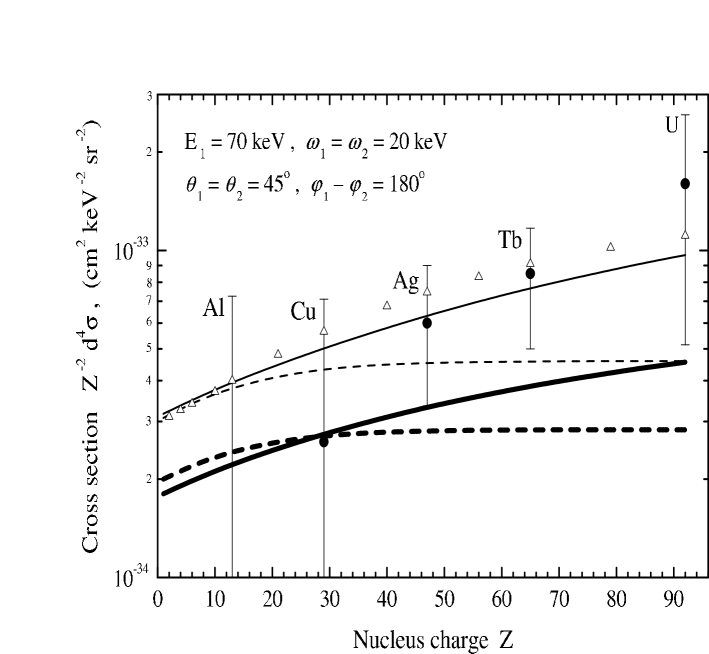
Figure 2: Dependence of $Z^{-2}\,{\rm d}^{4}\sigma_{\omega_{1}\omega_{2}}(\Omega_{1},\Omega_{2})$ on the nucleus charge $Z$. The incoming electron energy, the energies of the photons and the geometry of the emission are as indicated. Filled circles with the error bars are the experimental data from [29]. Solid lines correspond to the relativistic (thick line) and non-relativistic (thin line) ‘delta’-approximations. Dashed lines are used for the dependences obtained within the framework of relativistic (thick line) and non-relativistic (thin line) Born-Elwert approximations. Triangles present the results of the exact non-relativistic non-dipole approximation [4].

The results in all graphs refer to the com planar geometry when the vectors ${\bf p}_{1}$, ${\bf k}_{1}$ and ${\bf k}_{2}$ lay in the same plane. The emission angles $(\theta_{1,2},\varphi_{1,2})$, are measured with respect ${\bf p}_{1}$. Because of the axial symmetry the differential cross section ${\rm d}^{4}\sigma/({\rm d}\omega_{1}{\rm d}\omega_{2}{\rm d}\Omega_{1}{\rm d}\Omega_{2})\equiv{\rm d}^{4}\sigma_{\omega_{1}\omega_{2}}(\Omega_{1},\Omega_{2})$ depends on the difference $(\varphi_{1}-\varphi_{2})$ but not on the angles $\varphi_{1}$ and $\varphi_{2}$ separately.

The kinetic energy $\varepsilon_{1}=70$ keV, the photon energies and the geometry of the radiation correspond to the experimental conditions [29, 30, 31, 32].

Figure 3: Calculated cross section ${\rm d}^{4}\sigma_{\omega_{1}\omega_{2}}(\Omega_{1},\Omega_{2})$ as a function of $Z$ versus the experimental data from [30]. Solid lines correspond to the relativistic (thick lines) and non-relativistic (thin lines) ‘delta’-approximations. The results of relativistic plane-wave Born and relativistic Born-Elwert approximations are drawn with the short-dashed and the long-dashed lines, respectively. The energies $\varepsilon_{1}$, $\omega_{1,2}$ and the emission geometry are as indicated.

Figure 4: The calculated cross section ${\rm d}^{4}\sigma_{\omega_{1}\omega_{2}}(\Omega_{1},\Omega_{2})$ as a function of $\omega_{2}$ versus the experimental data [30] for a 70 keV electron collision with an Au atom ($Z=79$). Solid lines correspond to the relativistic (thick line) and non-relativistic (thin line) ‘delta’-approximations. Short-dashed line represents the relativistic plane-wave Born approximation, the long-dashed one stands for the correction due to the Elwert factor (35).

Numerical calculation of the relativistic amplitudes was carried out within the framework of the ‘delta’-approximation and using the FSM wavefunctions. The analogous non-relativistic calculations were performed with the exact Coulomb wavefunctions. The results of relativistic Born calculations presented in the figures were obtained by programming the formulae presented in [5]. The curves corresponding to the relativistic Born-Elwert approximation represent the relativistic Born curves corrected by the Elwert factor [60] (we used its relativistic analogue proposed in [64]):

$$f_{\rm Elw}={p_{1}\over p_{2}}\,{1-\exp{(-2\pi\xi_{1})}\over 1-\exp{(-2\pi\xi_{2})}}$$ (35)

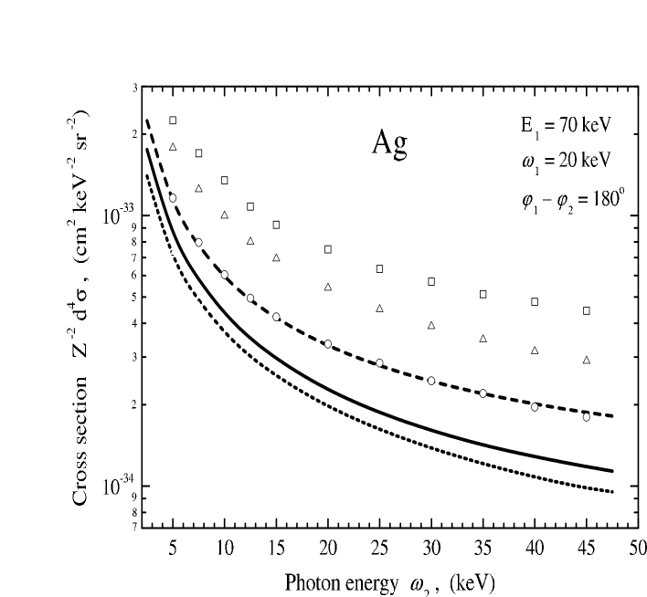
Figure 5: Results from the relativistic ‘delta’-approximation theory versus the exact non-relativistic calculations [4] for $Z^{-2}\,{\rm d}^{4}\sigma_{\omega_{1}\omega_{2}}(\Omega_{1},\Omega_{2})$ in a 70 keV electron collision with an Ag atom (${Z=47}$). The sets of curves (the ‘delta’-approximation) and symbols (the exact non-relativistic results) correspond to different emission geometries: (a) solid line and triangles are used for $\theta_{1}=\theta_{2}=30^{\circ}$, (b) long-dashed line and squares for $\theta_{1}=\theta_{2}=45^{\circ}$, and (c) short-dashed line and circles for $\theta_{1}=\theta_{2}=90^{\circ}$.

In figures 2–4 we compare the results of calculation of 2BrS cross section obtained within the framework of relativistic ‘delta’-approximation with the available experimental data [29, 30, 31, 32] and the the results from other theories. The latter include the exact non-relativistic non-dipole treatment of the 2BrS process in a point Coulomb field [4, 17], the non-relativistic non-dipole ‘delta’-approximation [3], and the relativistic plane-wave Born approximation with and without the correction factor (35). The calculations within the framework of the non-relativistic dipole approximations, although having been carried out, are not presented here. This is because, as it is known [3, 41], the dipole-photon scheme, which neglects the correction terms of the leading order $v/c$, strongly underestimates the magnitude of the 2BrS cross section.

One of the conclusions which can be drawn on the basis of the data presented in figures 2–4 is that the relativistic effects result in a decrease of the magnitude of the cross section. This is clearly seen if one compares the dependences obtained by using the relativistic (thick line) and non-relativistic (thin line) ‘delta’-approximations, which are presented in figure 2. Qualitatively, the influence of the relativistic corrections could be illustrated in terms of classical electrodynamics as follows. Apart from the spin-related effects, the general consequence of a movement with relativistic velocity is the dependence of mass of a projectile on its velocity, which leads to the increase of the mass as $m=m_{0}\,(1-v^{2}/c^{2})^{-1/2}$ ($m_{0}$ is the rest mass). This effect reduces the magnitude of the projectile’s acceleration, which defines the intensity of radiation.

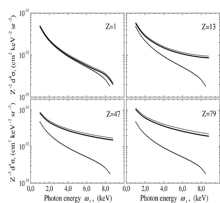
Figure 6: Comparison of the results of relativistic ‘delta’-approximation with the exact non-relativistic calculations with accounting for radiation retardation [17] of 2BrS cross section $Z^{-2}\,{\rm d}^{4}\sigma_{\omega_{1}\>\!\omega_{2}}(\Omega_{1},\Omega_{2})$ as function of energy of second emitted photon $\omega_{2}$. Presented four graphs correspond to collision of $10$ keV electron with four different atomic targets with ${Z=1,\,13,\,47,\,79}$. The energy of the first emitted photon $\omega_{1}=1$ keV and emission geometry $\theta_{1}=\theta_{2}=45^{\rm o}$, $\varphi_{1}-\varphi_{2}=180^{\rm o}$ are the same for all graphs. Results of relativistic ‘delta’-approximation are given by thick solid line. For results of non-relativistic exact calculations the thin solid line is used. Relativistic plane-wave Born curves are plotted by dashed line.

Presented results show that the relativistic ‘delta’-approximation, on the whole, reproduces quite well the available experimental data. However, there are two exceptions. In figure 2 in the range $Z\sim 100$ the calculated values underestimate the experimental data. The possible explanation of this discrepancy is in the inadequacy of the FSM approach in the limit $\alpha Z\sim 1$, The second example of a strong deviation between the theory and the experiment is seen in figure 4 at the tip-end of the spectrum. However, in this case, the discrepancy may be due to the experimental error, since the experimental data for $\omega_{2}=50$ keV lies far above all theoretical predictions.

In figure 5 we compare the predictions obtained within relativistic ‘delta’-approximation scheme with the results of the exact non-relativistic theory (the retardation included) [4]. It was demonstrated in the cited paper in the non-relativistic domain the ‘delta’-approximation is in a good agreement with the exact calculations. The account for the relativistic effects leads to the decrease in the cross section magnitude. This influence has been already mentioned above. We note also that this decrease is dependent on the geometry of the emission. The nature of this feature is not fully clear at present, and we believe to get the explanation as soon as the exact relativistic results will become available.

For the lower values of the projectile energy the influence of the relativistic corrections is less pronounced. This is demonstrated by figure 6 where the results of the relativistic ‘delta’-approximation (thick solid lines) for a 10 keV electron are compared with the exact non-relativistic non-dipolar calculations (thin solid lines) presented in [17]. Let us point out that the non-relativistic theory based on the ‘delta’-approximation produces the results (not plotted in the figure) which practically coincide with the thin lines for all elements presented. The difference between the thick and thin solid curves increases with the atomic number $Z$. Although the exact nature of the difference can be established when the exact relativistic theory of the effect becomes available, some part of it can be attributed to the use of the FSM wavefunctions which accuracy also decreases with $Z$.

For the sake of comparison in figure 6 we present the curves corresponding to the relativistic plane-wave Born approximation (dotted lines). It is clearly seen that the simpler theory becomes absolutely inapplicable in the range of medium and large $Z$ values.

On the whole, we may state that the developed approach is adequate for the description of 2BrS process and is an efficient tool for numerical analysis of the characteristics of the process (the spectral and spectral-angular intensities of the radiation). The results obtained within the ‘delta’-approximation (both relativistic and non-relativistic) describe quite well the behaviour of 2BrS cross sections over wide ranges of energies of the projectile electron and the photons and of atomic numbers $Z$. The influence of the relativistic effects increases with $\varepsilon_{1}$ and $Z$, and they must be accounted for in addition to the radiation retardation effect.

4 Conclusions

Basing on the numerical results presented above, we regard the developed approach as more reliable than the simpler relativistic theories. Within the framework of the ‘delta’-approximation the analytical structure of the 2BrS amplitude is simplified considerably. Additionally, this method allowed, for the first time, to carry out numerical analysis of the two-photon free-free transitions in relativistic domain beyond the plane wave Born approximation. The method is easily generalized to the case of a $n$-photon free-free transition.

Nevertheless, despite the (relative) simplicity and the efficiency of the outlined formalism, by no means does it solve in full the problem of the free-free relativistic transitions. The exact relativistic treatment of the process is still unavailable. This task is difficult from the analytical and the computational viewpoints. The direct evaluation of the amplitude by means of the partial wave expansion of the initial/final states wavefunction, the Green’s function and the multipole expansions for the emitted photons seems hardly to be implemented in the nearest future.

However, we are more optimistic on the prospects of two other approaches. The first one is based on the exact relativistic treatment of the 2BrS process within the framework of the FSM approximation, where one can construct, in addition to the wavefunctions, a practically useful form for the Green’s function (see [42]). The second approach is based on the Sternheimer-Dalgarno-Lewis method [58, 59] for the calculation of two-photon transition amplitude between two states of a continuous spectrum. The work in these directions is being carried out.

References

References

- [1] Korol, A. V., 1994. J. Phys. B 27, 155-174.
- [2] Korol, A. V., 1995. J. Phys. B 28, 3873-3887.
- [3] Korol, A. V., 1996. J. Phys. B 29, 3257-3276.
- [4] Korol, A. V., 1997. J. Phys. B 30, 413-438.
- [5] Fedorova, T. A., Korol, A. V., Solovjev, I. A., 2000. J. Phys. B 33, 5007-5024.
- [6] A. Maquet. A., Véniard, V., Marian, T. A., 1998. J. Phys. B 31, 3743-3764.
- [7] Ehlotzky, F., Jaroń, A., Kamisńki, J. Z., 1998. Phys. Rep. 297, 63-153.
- [8] Korol, A. V., Solov’yov, A. V., 1997. J. Phys. B 30, 1105-1150.
- [9] Berestetskii, V. B., Lifshitz, E. M., Pitaevskii, L.P., 1982. Quantum Electrodynamics. Pergamon, Oxford.
- [10] Akhiezer, A. I., Berestetskii V. B., 1969. Quantum Electrodynamics. Nauka, Moscow.
- [11] Rosenberg, L., 1994. Phys. Rev. A 49, 4770-4777.
- [12] Korol, A.V., 1995. Nucl. Instrum. Methods B 99, 160-162.
- [13] Florescu, V., Djamo, V., 1986. Phys. Lett. 119A, 73-76.
- [14] Véniard, V., Gavrila, M., Maquet, A., 1987. Phys. Rev. A 35, 448-451.
- [15] Gavrila, M., Maquet, A., Véniard V., 1990. Phys. Rev. A, 42, 236-247.
- [16] Dondera, M., Florescu, V., 1993. Phys. Rev. A 48, 4267-4271.
- [17] Dondera, M., Florescu, V., 1998. Phys. Rev. A 58, 2016-2022.
- [18] Véniard, V., Piraux, B., 1990. Phys. Rev. A 41, 4019-4034.
- [19] Blaha, M., Davis, J. 1995. Phys. Rev. A 51, 2308-2315.
- [20] Mercouris, N., Komninos, Y., Dionissopoulou, S., Nicolaidest, C. A. 1996. J. Phys. B 29, L13-L19.
- [21] Gribakin G. F., Ivanov V. K., Korol A. V., Kuchiev M. Yu., 1999. J. Phys. B 32, 5463-5478; 2000. ibid. 33, 821-828.
- [22] Korol, A. V., 1994. J. Phys. B 27, 4765-4777.
- [23] Manakov, N. L., Marmo, S. I., Fainstein, A. G., 1995. JETP 81, 860 -877.
- [24] Krylovetskii, A. A., Manakov, N. L., Marmo, S. I., Starace, A. F. 2002. JETP 95, 1006-1032.
- [25] Florescu, A., Florescu, V., 2000. Phys. Rev. A 61, 033406.
- [26] Altman, J. C., Quarles, C. A., 1985, Phys. Rev. A 31, 2744; 1985, Nucl. Instrum. Methods A 240, 538.
- [27] Lehtihet, H. E., Quarles, C. A., 1989, Phys. Rev. A 39, 4274.
- [28] Hippler, R., 1991, Phys. Rev. Lett. 66, 2197.
- [29] Kahler, D. L., Liu, J., Quarles, C. A., 1992. Phys. Rev. A 45, R7663-R7666; 1992. Phys. Rev. Lett. 68, 1690-1693.
- [30] Liu, J., Quarles, C. A., 1993. Phys. Rev. A 47, R3479-R3482.
- [31] Liu, J., Kahler, D. L., Quarles, C. A., 1993. Phys. Rev. A 47, 2819-2826.
- [32] Quarles, C. A., Liu, J., 1993. Nucl. Instrum. Methods B 79, 142.
- [33] Hippler, R., Schneider, H., 1994, Nucl. Instrum. Methods A 87, 268.
- [34] Smirnov, A. I., 1977. Sov. Phys. – Nucl. Phys. 25, 548-552.
- [35] Ghilencea, D., Toader, O., Diaconu, C. 1995. Romanian Rep. in Phys. 47, 185-196.
- [36] Gavrila, M., Maquet, A., Véniard, V., 1985. Phys. Rev. A 32, 2537-2540 (Erratum: 1986. ibid. 33, 2826).
- [37] Korol, A. V., 1993. J. Phys. B 26, 3137-3145.
- [38] Amusia, M.Ya., Korol, A.V., 1993, Nucl. Instrum. Methods B 79, 146.
- [39] Kracke, G., Alber, G., Briggs, J.S., Maquet, A., 1993, J. Phys. B 26, L561.
- [40] Kracke, G., Briggs, J. S., Dubois, A., Maquet, A., Véniard, V., 1994, J. Phys. B 27, 3241.
- [41] Dondera, M., Florescu, V., Pratt, R. H., 1996. Phys. Rev. A 53, 1492.
- [42] Gorshkov, V. G., 1964. Zh. Eksp. Teor. Fiz. 47, 1984-1988.
- [43] Florescu, V., Gavrila, M., 1976. Phys. Rev. A 14, 211-235.
- [44] Wong, M. K. F., Yeh, E. H. Y., 1985. J. Math. Phys. 26, 1701-1710.
- [45] Zapryagaev, S. A., Manakov, N. L., Palchikov, V. G., 1985. The Theory of One- and Two-Electron Multicharged Ions. Energoatomizdat, Moscow (in Russian).
- [46] Manakov, N. L., Ovsyannikov, V. D., Rappoport, L. P., 1986. Phys. Rep. 141, 319.
- [47] Mu, X., Crasemann, B., 1988. Phys. Rev. A 38, 4585-4596.
- [48] Florescu, V., Marinesku, M., Pratt, R.H., 1990. Phys. Rev. A 42, 3844-3851 (Erratum: 1991. ibid. 43, 6432).
- [49] Bergstrom, P.M. Jr., Surić, T., Pisk, K., Pratt, R.H., 1993. Phys. Rev. A 48, 1134-1162.
- [50] Manakov, N.L., Maquet, A., Marmo, S.I., Szymanovski, C., 1998. Phys. Lett. 237A, 234-239.
- [51] Szmytkowski, R., 2002. Phys. Rev. A 65, 012503.
- [52] Yakhontov, V., 2003. Phys. Rev. Lett. 91, 093001.
- [53] Szmytkowski, R., Mielewczyk, K., 2004. J. Phys. B 37, 3961-3972.
- [54] Rosenberg, L., 1987. Phys. Rev. A 36, 4284-4289; 1990. ibid. 42, 5319-5327; 1991. ibid. 44, 2949-2954.
- [55] Gribakin, G. F., Ivanov, V. K., Korol, A. V., Kuchiev, M. Yu., 1999, J. Phys. B 32, 5463; 2000, ibid. 33, 821.
- [56] Varshalovich, D. A., Moskalev, A. N., Khersonskii, V. K., 1988. Quantum Theory of Angular Momentum. World Scientific, NY.
- [57] Geltman, S., 1996. Phys. Rev. A 53, 3473-3483.
- [58] Sternheimer, R. M., 1954. Phys. Rev. 96, 951-968.
- [59] Dalgarno, A., Lewis, J.T., 1955. Proc. R. Soc. London A 223, 70-74.
- [60] Elwert, G., Haug, E., 1969. Phys. Rev. 183, 90-105.
- [61] Shaffer, C.D. and Pratt, R. H., 1997. Phys. Rev. A 56, 3653-3658.
- [62] Hostler, L., 1964. J. Math. Phys. 5, 591.
- [63] Nordsieck, A., 1954. Phys. Rev. 93, 785-787.
- [64] Avdonina, N. B., Pratt, R. H., 1999, J. Phys. B 32, 4261-4276.