Cold collisions in dissipative optical lattices

Abstract

The invention of laser cooling methods for neutral atoms allows optical and magnetic trapping of cold atomic clouds in the temperature regime below $1$mK. In the past, light-assisted cold collisions between laser cooled atoms have been widely studied in magneto-optical atom traps (MOTs). We describe here theoretical studies of dynamical interactions, specifically cold collisions, between atoms trapped in near-resonant, dissipative optical lattices. The extension of collision studies to the regime of optical lattices introduces several complicating factors. For the lattice studies, one has to account for the internal substates of atoms, position dependent matter-light coupling, and position dependent couplings between the atoms, in addition to the spontaneous decay of electronically excited atomic states. The developed one-dimensional quantum-mechanical model combines atomic cooling and collision dynamics in a single framework. The model is based on Monte Carlo wave-function simulations and is applied when the lattice-creating lasers have frequencies both below (red-detuned lattice) and above (blue-detuned lattice) the atomic resonance frequency. It turns out, that the radiative heating mechanism affects the dynamics of atomic cloud in a red-detuned lattice in a way that is not directly expected from the MOT studies. The optical lattice and position dependent light-matter coupling introduces selectivity of collision partners. The atoms, which are most mobile and energetic, are strongly favored to participate in collisions, and are more often ejected from the lattice, than the slow ones in the laser parameter region selected for study. Consequently, the atoms remaining in the lattice have a smaller average kinetic energy per atom than in the case of non-interacting atoms. For blue-detuned lattices, we study how optical shielding emerges as a natural part of the lattice and look for ways to optimize the effect. We find that the cooling and shielding dynamics do not mix and it is possible to achieve efficient shielding with a very simple arrangement. The simulations are computationally very demanding and would obviously benefit from the simplification schemes. We present some steps to this direction by showing how it is possible to calculate collision rates in near-resonant lattices in a fairly simple way. The method can then be used to combine quantum-mechanical and semiclassical models for cold collision studies in optical lattices.

1 Introduction

It has been known for a long time that light can exert a force on material objects. The first experiments which showed the effect of the radiation pressure of an electromagnetic field on matter predicted by Maxwell were done at the beginning of the last century [1]. Since then, the success of applying the light force in a controlled way to cool gaseous atomic clouds to temperatures around, and even below, the $\mu$K range has given a huge impetus to the field of cold atomic physics.

Laser cooling and trapping of neutral atoms has been a very rapidly developing field of physics since the mid-eighties when experimentalists succeeded for the first time to optically trap laser cooled atoms [2]. More recent milestones include the experimental realizations of atomic Bose-Einstein condensate (BEC) [3], Fermi degenerate dilute quantum gas [4], superfluid–Mott-insulator phase transition in optical lattices [5], molecular BEC [6], and evidence for superfluidity in an atomic Fermi gas [7].

In general, the slow motion of the laser cooled atoms changes drastically the collision dynamics of the atoms compared to room temperature gases. The collisions may become inelastic and the research on cold collisions in magneto-optical traps (MOTs) has shown how the collisions consequently limit the densities and temperatures of atomic gases in MOTs [8, 9]. The purpose of this article is to describe and review the work which has been done to extend the regime of cold collision studies to optical lattices.

This tutorial gives a simple introduction to one specific cooling and trapping scheme for neutral atoms: near-resonant, dissipative optical lattices, and concentrates on the description of light-assisted cold collisions in this system. A thorough introduction into the field of laser cooling, trapping, and optical lattices can be found from a text book [10], various review articles [11, 12, 13, 14, 15, 16, 17, 18], and summer school lecture notes [19, 20, 21]. Cold collision theories and experiments are reviewed in detail in Refs. [8, 9, 22].

The article is organized as follows. Section 2 gives a short introduction to near-resonant, dissipative optical lattices. We describe both the red- and blue-detuned lattices. The latter are sometimes in the literature referred also as gray or dark optical lattices due to the reduced number of scattered photons compared to ”bright” red-detuned optical lattices. Section 3 describes the basic cold collision mechanisms in the presence of a near-resonant light, radiative heating by the red-detuned light and optical shielding by the blue-detuned light. Section 4 shows a formulation of the cold collision problem in optical lattices and overviews the central results. Finally, we conclude with a few remarks in Section 5.

2 Optical lattices

A disordered cold atomic gas can be arranged into an ordered structure by periodic optical potentials which are created with suitably chosen set of interfering laser beams [12, 14, 15, 16, 17, 18]. An optical lattice formed by optical potentials does not only trap the atoms, but it is also able to cool them via optical pumping and Sisyphus mechanism [23, 24].

The typical temperature range for alkali metal atoms cooled and trapped in optical lattices falls between the so called Doppler limit $T_{d}$ and recoil limit $T_{r}$. The Doppler limit gives lower bound for Doppler cooling, the main cooling mechanism in MOTs, and can be written as

$$T_{d}=\hbar\Gamma/2k_{B},$$ (1)

where $\hbar$ is Planck’s constant $h$ divided by $2\pi$, $\Gamma$ the atomic linewidth, and $k_{B}$ Boltzmann’s constant. The recoil limit in turn describes the lower bound for polarization gradient cooling mechanisms, and $T_{r}$ corresponds to the amount of energy of single photon absorption or emission recoil, and is given by

$$T_{r}=\left(\hbar k_{r}\right)^{2}/Mk_{B}.$$ (2)

Here $k_{r}$ is the wavenumber of the cooling lasers, and $M$ the mass of an atom. The corresponding energy unit

$$E_{r}=\left(\hbar k_{r}\right)^{2}/2M,$$ (3)

is consequently called recoil energy. A typical alkali element used for laser cooling, Cs, has $T_{d}=120\mu$K and $T_{r}=0.2\mu$K.

The modern work on optical lattices was preceded by the proposal of Letokhov to trap cold atoms in one dimension by using a standing light wave [25], and accompanied by the experiment of Burns et al. who created crystal structures of microscopic dielectric objects suspended in liquid by standing light waves [26]. Because of the purity and ease of control in optical lattices, the trapped atoms are almost ideal for the study of phenomena which are familiar from solid-state physics. A few examples of these phenomena, which have been realized in experiments, include the Bragg scattering [27, 28], Bloch oscillations [29], and Wannier-Stark ladders [30]. Other interesting observations include the quantum Zeno effect [31] and dynamical tunneling [32]. During the last few years, the amount of research exploiting optical lattices has hugely increased. This is mainly because now it is possible to load far-off resonant optical lattices with Bose-Einstein condensates (BECs). This has led to the observation of superfluid–Mott-insulator phase transition in far-detuned optical lattices [5] which paved the way e.g. to the creation of multiparticle entanglement by exploiting controlled collisions [33]. For dissipative optical lattices, a so called double lattice creates interesting prospects for the future studies [34]. In a double lattice, the atoms on two ground hyperfine states can be trapped and moved in a controllable way with respect to each other. This opens a new avenue to study inelastic cold collisions in the presence of near-resonant light in dissipative lattices.

2.1 Red-detuned dissipative optical lattices

The simplest case of cooling in optical lattices can be described by using the atomic level structure with the ground state angular momentum $J_{g}=1/2$ and the excited state $J_{e}=3/2$ [23]. A single atom has two ground state sublevels $|g_{\pm 1/2}>$ and four excited state sublevels $|e_{\pm 3/2}>$ and $|e_{\pm 1/2}>$, where the half–integer subscripts indicate the quantum number $m$ of the angular momentum along the $z$ direction. This is shown in Fig. 1 with the appropriate squares of the Clebsch-Gordan coefficients which describe the relative strengths of the light-induced couplings between the various levels.

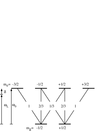
Figure 1: The level structure of a single atom for a red-detuned lattice. The squares of the Clebsch-Gordan coefficients for various transitions are shown, and the laser frequency $\omega_{L}$ is detuned a few atomic linewidths below the atomic resonance frequency $\omega_{0}$ for efficient Sisyphus cooling. The detuning of the laser is described by $\delta=\omega_{L}-\omega_{0}$.

2.1.1 Sisyphus cooling

The laser field consists of two counter–propagating beams along the $z$-axis with orthogonal linear polarizations and with frequency $\omega_{L}$. The total field has a polarization gradient in one dimension and reads (with suitable choices of phases of the beams and origin of the coordinate system)

$${\bf E}(z,t)={\cal E}_{0}({\bf e}_{x}e^{ik_{r}z}-i{\bf e}_{y}e^{-ik_{r}z})e^{-i\omega_{L}t}+c.c.,$$ (4)

where ${\cal E}_{0}$ is the amplitude and $k_{r}$ the wavenumber. With this field, the polarization changes from circular $\sigma^{-}$ to linear and back to circular in the opposite direction $\sigma^{+}$ when $z$ changes by $\lambda_{L}/4$ where $\lambda_{L}$ is the wavelength of the lasers. The periodic polarization gradient of the laser field is reflected in the periodic light shifts, i.e., AC–Stark shifts, of the atomic sublevels creating the optical lattice structure. Figure 2 displays a schematic view of the optical potentials and shows how the lattice wells coincide with the points of pure circular polarization of the light field.

When the atomic motion occurs in a suitable velocity range, the optical pumping of the atom between the ground state sublevels reduces the kinetic energy of the atom [23]. After several cooling cycles the atom localizes into an optical potential well, i.e., into an optical lattice site. Figure 3 shows the optical pumping cycles between the ground state sublevels and the oscillations of the atomic wave packet after localization into a lattice site.

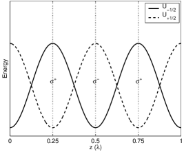
Figure 2: Schematic view of the optical potentials for the two ground state Zeeman sublevels in a red-detuned lattice with the atomic level structure $J_{g}=1/2,J_{e}=3/2$. The lattice structure is created due to the periodic polarization gradient of the laser field, and the points of pure circular polarization are indicated by dotted lines.

The intensity of the laser field and the strength of the coupling between the field and the atom is described by the Rabi frequency

$$\Omega=2d{\cal E}_{0}/\hbar,$$ (5)

where $d$ is the atomic dipole moment of the strongest transition between the ground and excited states. The detuning of the laser field from the atomic resonance is given by

$$\delta=\omega_{L}-\omega_{0},$$ (6)

where $\omega_{0}$ is the atomic resonance frequency. As a unit for $\Omega$ and $\delta$ the atomic linewidth $\Gamma$ is commonly used.

The Hamiltonian for a single atom moving in the laser field given in Eq.(4) is after the rotating wave approximation

$$H=\frac{p^{2}}{2M}-\hbar\delta P_{e}+{V}.$$ (7)

Here, $p^{2}/{2M}$ is the kinetic energy, $\delta$ the detuning of the laser, $P_{e}=\sum_{m=-3/2}^{3/2}|e_{m}\rangle~{}\langle e_{m}|$ is the projection operator onto the excited state, and the interaction between a single atom and the field is

$${V} = -i\frac{\hbar\Omega}{\sqrt{2}}\sin(k_{r}z)\left\{|e_{3/2}\rangle\langle g_{1/2}|+\frac{1}{\sqrt{3}}|e_{1/2}\rangle\langle g_{-1/2}|\right\}$$ (8)

$$+\frac{\hbar\Omega}{\sqrt{2}}\cos(k_{r}z)\left\{|e_{-3/2}\rangle\langle g_{-1/2}|+\frac{1}{\sqrt{3}}|e_{-1/2}\rangle\langle g_{1/2}|\right\}+H.c.,$$

where $z$ is the position operator of the atom. The spatially modulated optical potentials read

$$U_{-}=U_{0}\sin^{2}(k_{r}z),$$

$$U_{+}=U_{0}\cos^{2}(k_{r}z),$$ (9)

for ground states $m_{g}=-1/2$ and $m_{g}=+1/2$, respectively [35]. Here, $U_{0}$ is the modulation depth of the lattice.

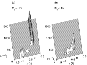
Figure 3: Sisyphus cooling and the localization of an atom into the optical lattice. A possible time evolution for a single atom wave packet is shown for two ground state Zeeman levels: (a) $m_{g}=-1/2$ and (b) $m_{g}=+1/2$. The result shows the optical pumping cycles and the localization of a single atom into the optical lattice. The discontinuous changes between the two ground states are due to quantum jump events from the excited state (not shown), selected to happen randomly with an appropriately weighted probability. If the run is repeated, the jumps would appear at different times.

2.1.2 Localization in lattice

When the steady state is reached after a certain period of cooling, atoms are, to a large extent, localized into the lattice sites. The optical lattice is in the oscillating regime if the atom completes on average more than one oscillation in the site before being optically pumped to a neighboring site. For less than one average oscillation per site, the lattice is in the jumping regime. The laser parameters $\Omega$ and $\delta$ determine in which of the regimes the lattice is in [35]. It must be noted that tight localization and occupation of the lowest vibrational levels of a periodic lattice potential increases the optical pumping time, and the time of localization within a single lattice site becomes longer compared to the semiclassical values [23]. Since we are mainly interested in the case when the two atoms undergo an intra-well collision, the chosen parameters in our work correspond to the jumping regime of the lattice.

In our studies, the laser field is detuned a few atomic linewidths below [36, 37, 38] or above [39] the atomic transition. The most typical detuning range we use is $3\Gamma\leq\delta\leq 10\Gamma$ towards the oscillating regime. Whereas the most common range in the dissipative lattice experiments done so far is slightly higher, $5\Gamma\leq\delta\leq 20\Gamma$, and in the oscillating regime.

2.2 Blue-detuned dissipative optical lattices

Two counterpropagating orthogonally polarized blue-detuned ($\delta>0$) laser beams can efficiently cool down atoms which have the level structure $J_{e}=J_{g}$ or $J_{e}=J_{g}-1$ [17]. The lowest position-dependent eigenstate of the system is flat in this case and is not directly coupled to the light field at any point of space. Thus, despite of the cooling, the atoms are not efficiently trapped.

The problem can be circumvented by the use of either transverse [40] or longitudinal [41] magnetic fields with respect to the laser propagation axis. We have used for collision studies the proposal of Grynberg and Courtois with a magnetic field along the laser axis [42], see below. We note that there exists also possibilities to create blue-detuned gray lattices by all-optical means [43, 44].

2.2.1 Grynberg-Courtois gray optical lattice

An applied longitudinal magnetic field removes the degeneracy of the atomic states of blue-detuned optical molasses mentioned above, and produces the necessary spatial modulation for the optical potentials and the lattice structure [17].

In general, the atomic states are now Zeeman shifted by the magnetic field, and light shifted by the laser. The ratio between the two shifts can be varied by changing the intensity of the laser or the strength of the magnetic field. Obviously, the two extreme regimes are: a) the Zeeman shift is small compared to the light shift b) the light shift is small compared to the Zeeman shift.

In case a), where the light shift dominates, the behavior of the lattice is paramagnetic and the increasing magnetic field strength increases the lattice modulation depth. When the Zeeman shift dominates in the case b), the laser field produces perturbations to the Zeeman shifted states. The situation resembles now the traditional Sisyphus cooling scheme and the lattice is in the antiparamagnetic regime.

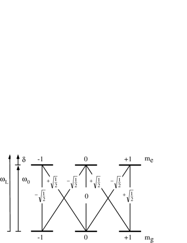
Figure 4: The level structure of a single atom for a blue-detuned lattice with the Clebsch-Gordan coefficients of corresponding transitions. This structure corresponds to particular hyperfine states of ⁸⁷Rb and can be used for efficient cooling and trapping of atoms in the Grynberg-Courtois blue-detuned lattice in the antiparamagnetic regime [42].

We have done our collision studies in this antiparamagnetic regime. See Fig. 4 for the used atomic level configuration $J_{e}=J_{g}=1$ and Fig. 5 for the corresponding optical lattice structure. We label the three ground state sublevels with $|g_{\pm 1}>,|g_{0}>$, and the three excited state sublevels with $|e_{\pm 1}>,|e_{0}>$, where the integer subscripts indicate the angular momentum projection quantum number $m$ along the $z$-axis. Because the standing laser field has only circular components, and the Clebsch-Gordan coefficient between $m_{e}=0$ and $m_{g}=0$ states is zero, the atoms are rapidly pumped to the $\Lambda$ subsystem of the whole state structure; thus, in this level configuration, the atoms are trapped to the ground substates which have an angular momentum quantum number $m_{g}=-1$ and $m_{g}=+1$. The excited state with $m_{e}=0$ provides a way for cooling optical pumping cycles between the two trapping ground substates.

After the rotating wave approximation the Hamiltonian for the atomic system interacting with the laser field given in Eq. (4) is

$$H=\frac{p^{2}}{2M}-\hbar\delta P_{e}+{V}+{U}.$$ (10)

Here, $P_{e}=\sum_{m=-1}^{1}|e_{m}\rangle~{}\langle e_{m}|$ is the projection operator, and the interaction between a single atom and the field is

$$V = i\frac{\hbar\Omega}{\sqrt{2}}\sin(kz)\left\{|e_{0}\rangle~{}\langle g_{-1}|+|e_{1}\rangle\langle g_{0}|\right\}$$ (11)

$$+\frac{\hbar\Omega}{\sqrt{2}}\cos(kz)\left\{|e_{-1}\rangle\langle g_{0}|+|e_{0}\rangle\langle g_{1}|\right\}+H.c.,$$

where $z$ is the position operator of the atom, and the Rabi frequency $\Omega$ is defined as

$$\Omega=2d{\cal E}_{0}/\sqrt{2}\hbar.$$ (12)

The interaction with a magnetic field in Eq. (10) is

$${U}=\sum_{i}m_{i}\hbar\Omega_{B_{i}}|i\rangle\langle i|,$$ (13)

where the sum over $i$ includes all the ground and excited states, and the Zeeman shift factors $\Omega_{B_{i}}$ for the two trapping ground substates $m=\pm 1$ are equal.

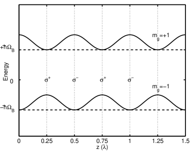
Figure 5: Schematic view of the optical potentials for the two trapping ground state Zeeman sublevels in a blue-detuned lattice. The periodic polarization gradient of the laser field creates the lattice structure and the points of circular polarizations are indicated by $\sigma^{+}$ and $\sigma^{-}$. The dashed lines give the Zeeman shifted energy levels which the light field modifies.

The level structure which we have used in our studies for a blue-detuned lattice can be found in ⁸⁷Rb, which has $F=1$ hyperfine states for both the 5S_1/2 ground state and the 5P_1/2 excited state. This is actually the element and the level scheme which has been used in the blue-detuned lattice experiment of Hemmerich et al. [40], even though in their case the lattice structure and the orientation of the magnetic field differs from what is presented here.

The reason for the choice we have made for the used level structure and an antiparamagnetic regime of the Grynberg-Courtois lattice is in their simplicity. The cooling mechanism resembles the traditional Sisyphus cooling, making it more relevant to compare the results between the red and blue-detuning studies. Moreover, it is necessary to use only three levels of the $\Lambda$-subsystem instead of all the six levels of a single atom. Thus the number of product state basis vectors for interaction studies between the atoms can be reduced in the blue-detuned case. This reduces the computational resource requirements and speeds up the simulations when compared to red-detuned case (which has to use all the six substates of a single atom for the interaction studies). Thus for blue-detuned lattices it is easier to make a wider exploration of parameter space, if required.

2.3 Basic theoretical approaches

Because of the polarization gradients, the laser couples the multitude of Zeeman substates of the atom in a position dependent way and the spontaneous emission caused by the coupling to the vacuum plays a crucial role in the optical pumping process. Thus, to describe the atomic motion in optical lattices one has to solve the problem of a multi-level atom coupled to a monochromatic laser field and to a quantized electromagnetic environment in its vacuum state.

It is possible to treat the external laser field classically since the fields which are considered weak from the lattice point of view still contain a large number of photons. Typical laser intensities used in experiments are a few mW/cm². The treatment of the interaction between a classical field and an atom is typically done with the rotating wave approximation, which neglects the terms that do not conserve the total energy.

The general form of the task is to solve the master equation for the density matrix $\rho$ of the atomic system

$$i\hbar\frac{d\rho}{dt}=\left[H,\rho\right]+{\cal L}_{rel}\left[\rho\right],$$ (14)

where $H$ is the system Hamiltonian, see Eqs. (7), (10), and ${\cal L}_{rel}$ includes the spontaneous emission part due to the coupling to the environment.

It is extremely difficult to find the exact analytical solution for this equation even in the case of the simplest atomic level schemes used for optical lattices. One can try to find approximations which allow an analytical treatment, or the combination of analytical and numerical calculations to Eq. (14). Another possibility is to simulate the optical lattice system on a computer, especially, simulations by the Monte Carlo wave-function (MCWF) method may provide a convenient way to obtain the solution of Eq. (14) [45, 46, 47, 48]. In the case of laser cooling, the combinations of analytical and numerical treatments can treat 2D case [49], but the 3D problem has been solved so far only by the MCWF simulations [50].

A common feature for analytical treatments of optical lattices is the adiabatic elimination of the excited states, thus reducing the number of the levels in the problem at hand [16]. One can then try to solve the master equation directly by numerical integration, introduce further approximations, or exploit the translational symmetry properties of the system [51].

The MCWF method was originally developed for the problems in quantum optics, where in many of the cases the direct quantum-mechanical solution of the system density matrix is very difficult or impossible to obtain. The method has been applied e.g. to the resonance fluorescence spectrum of 1D optical molasses [52] and to 3D laser cooling [50]. For more examples, see Ref. [48]. By now the method has also been applied outside the field of quantum optics, e.g. into transport problems in condensed matter physics [53]. The key idea of MCWF method is the generation of a large number of single wave function realizations which include stochastic quantum jumps of the system studied. The final result for the system density matrix and the system properties can then be calculated as ensemble averages of single realizations. Section 4.2 presents the method in more detail.

We have chosen for our collision studies in optical lattices the MCWF method since it has been a widely used benchmark method for various semiclassical theories for cold collisions in MOTs [54]. The method gives a full quantum-mechanical description of the atomic system (the external laser field is still described classically) and treats spontaneous decay in a rigorous way. A semiclassical version of the Monte Carlo (MC) method has also been developed for lattice studies [55] and has been applied e.g. to study anisotropic velocity distributions in 3D dissipative optical lattices [56]. This variant describes the external atomic degrees of freedom classically, and has limited applicability when the spread of the wave packet influences the dynamics of the system. This is the case when an atom is tightly localized into a lattice site and the spread of the packet affects essentially the optical pumping rate. Moreover, the semiclassical approach can not treat, e.g., the branching of the wave packet in optical lattice shown in Fig. 6. For the branching of the packets, see e.g. discussion in Ref. [57].

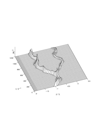
Figure 6: Branching of a wave packet. The time evolution of the total atomic wave packet in position space is shown. In addition to treating spontaneous decay in a rigorous way, the full quantum-mechanical MCWF method can also account for the branching of the wave packet in optical lattices.

3 Cold collisions between laser cooled atoms in the presence of near-resonant light

The thermal velocities of the atoms in a laser cooled gas are on the order of centimeters per second, roughly four orders of magnitude less than in a room temperature gas. Consequently, the collision dynamics is strikingly different within the two temperature regimes. The kinetic energies involved in the cold collision process are on the order or less than the energy of the atomic linewidth. For example, in the case of cesium the linewidth of a typical cooling transition is $2400$E_r and a typical collision energy is around $1600$E_r. Slow atomic motion indicates that the decay time of the excitation becomes small compared to the time scale of the total collision dynamics. This allows new phenomena in cold collision processes to affect the thermodynamics of the cold atomic cloud [8, 9].

A general categorization of the dynamical interactions between atoms can be made by considering collisions occurring between two ground state or between one ground and one excited state atom. Here we describe binary collisions between atoms of same element, i.e., a homonuclear diatomic molecule, and the emphasis is on the collisions between a ground and an excited state atom which is the relevant scheme for dissipative optical lattices.

In the presence of near-resonant light the excitation of a quasimolecule formed by the colliding atoms may occur at an extremely long range, even on the order of few thousands of Bohr radii a₀. Molecular potentials at these long ranges are usually labeled by the Hund’s case (c) notation, where the component of the total electronic angular momentum along the internuclear axis is a good quantum number. The electron clouds of the colliding atoms do not overlap at long range, and the dominant interaction between the atoms is the resonant dipole-dipole interaction. We give a description of the resonant dipole-dipole interaction in Section 4.1, earlier calculations for alkali-metals can be found in Refs. [58, 59].

The long range properties of molecular states and the sign of the detuning of the laser with respect the appropriate electronic transition define the possible consequences of collisions. A repulsive or an attractive character of the molecular potential at long range arises due to the relative orientation of the dipole moments of the colliding atoms. In the case of a red-detuned laser, the resonance or Condon point $r_{c}$, occurs for an attractive state. For a blue-detuned laser $r_{c}$ occurs for a repulsive state. Depending on the magnitude of the detuning and the strength of the coupling laser, off-resonant excitation to a non-resonant state may also play a role [39].

A very active research field of its own is the photoassociation of laser cooled atoms to molecules. Photoassociation is typically done by using a large red detuning of the laser so that free atom pair is excited at $r_{c}$ to a well defined bound molecular vibrational state. Especially photoassociation in an atomic Bose-Einstein condensate has attracted wide interest recently [60, 61, 62]. We will not discuss further photoassociation here but the reader can find presentations of the field e.g. from Refs. [9, 63].

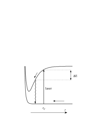
Figure 7: A schematic view of radiative heating of colliding atoms. The quasimolecule is excited at the Condon point $r_{c}$ and accelerated on the upper level before spontaneous decay terminates the process. The consequent kinetic energy gain is noted by $\Delta E$

3.1 Radiative heating by red-detuned light

With red-detuned light, the population of the quasimolecule formed by the two collision partners may get resonantly excited into an attractive excited state at the Condon point $r_{c}$ (see Fig. 7). The relative velocity of the atoms increases due to the acceleration on the attractive state until spontaneous emission terminates the process. When the atoms have again bounced apart due to the short range repulsion in the ground state, the pair may lose some of the gained kinetic energy in the reverse process, but to lesser degree. The overall effect is the heating of the colliding pair, and the escape of the atoms from the trap if the total gain in kinetic energy is large enough [9].

Figure 7 shows a semiclassical (SC) schematic view of the process. In some of the parameter regimes SC descriptions, such as the Landau-Zener level crossing model, can be used [54]. When the SC models fail, full quantum-mechanical methods are needed. For example, MCWF simulations [64, 65] can be used as a benchmark method for simpler analytical semiclassical calculations. It should be emphasized that it is difficult in SC models to account for population recycling, which means that once-decayed population may get re-excited in strong laser fields. A comparison between various methods and their application range is given in Ref. [54].

Most of the radiative heating studies done so far have used a simple two-state description with one ground and one excited molecular electronic state. An example of MCWF simulation results for MOT from Ref. [65] is shown in Fig. 8. The results demonstrate radiative heating via the spreading of the momentum distributions. The effect clearly becomes stronger as the initial collision momentum, i.e., cloud temperature, decreases. We emphasize that our lattice studies include many attractive and repulsive states simultaneously, see Section 4.1.

In addition to radiative heating, atoms may also escape from the trap by the fine-structure change mechanism. If the population survives on the excited state for small enough relative distance between the two atoms, the point where two fine-structure states have a crossing may be reached. Now, if the pair comes out from the collision in an energetically lower fine-structure state than the one in which they entered the collision, the pair gains kinetic energy by the amount corresponding to the fine-structure splitting of the atomic electronic states at large $r$. This energy difference is usually large compared to the trap depths, and consequently in this case the atoms escape from the trap [8, 9].

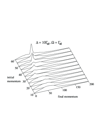
Figure 8: An example of a radiative heating study in MOT from Ref. [65]. The final momentum distributions for various initially Gaussian momentum distributions are shown. The initial momentum refers to the $\langle p\rangle$ of the narrow initial momentum distributions. The effects of radiative heating, the spreading of the distributions, and the momentum increase is clearly visible, especially for low initial relative momentum. For higher initial momentum some character of the initial distribution is still preserved in the post-collision distribution.

We deal in our studies with very small detunings, a few atomic linewidths only, and strong laser fields. It is therefore reasonable to assume that the effect of fine-structure changing collisions on the cloud temperature is very small compared to the effect of radiative heating processes, and we neglect the fine-structure change loss mechanism in our lattice studies. The assumption is also supported by the fact that there can be an order of magnitude difference between the fine-structure state crossing point and $r_{c}$ for the small detunings we have used.

3.2 Optical shielding by blue-detuned light

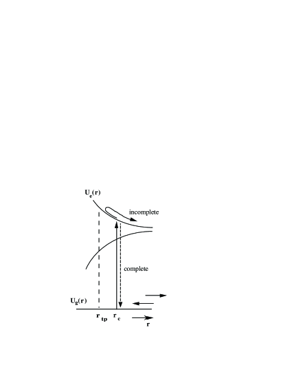
Figure 9: A schematic semiclassical presentation of optical shielding. The quasimolecule is excited resonantly to the repulsive molecular state $U_{e}$ at the Condon point $r_{c}$. Then it reaches the classical turning point $r_{tp}$, and is finally transferred back to the ground state $U_{g}$ when arriving at $r_{c}$ again. If the transfer back to the ground state is not complete, the atom pair may gain kinetic energy as it is further accelerated by the excited state potential. In this case shielding is incomplete and the collision is inelastic. If the population transfer between the states is adiabatic, shielding is complete and the collision between the atoms is elastic.

When blue-detuned light is used, the resonant excitation at the Condon point occurs to a repulsive excited quasimolecular state. This makes it possible to shield the atoms from close encounters [9], see Fig. 9. If the shielding is efficient, collisions between atoms may become completely elastic. The mechanism would obviously be useful for preventing loss of atoms in optical lattices formed with a near-resonant blue-detuned light.

In an optical shielding process, the resonantly excited quasimolecule population reaches the classical turning point on the repulsive excited state and the atoms begin to move apart again. The shielding becomes complete if all the population has been excited, no spontaneous decay has occurred, and all the population returns resonantly to the ground state at the Condon point. In this case, collisions become elastic (when photon recoil effects are ignored), and no heating or escape occurs due to the inelastic processes. Moreover, the ground state is emptied at a relatively long range, and no population reaches short distances where unwanted processes are possible, such as hyperfine state changing collisions. Thus, the possibility to use optical shielding in an efficient way allows to increase the occupation density of the dissipative lattice, in addition to the benefit of reducing the rate of scattered and reabsorbed photons and the consequent effects.

In the past the MCWF simulations have described the efficiency of the shielding process in a MOT by a shielding measure $P_{S}$, which essentially describes the flux of the ground state population to the short range beyond the Condon point $r_{c}$ [66, 67, 68], see Fig. 10. In the case of optical lattices, a more descriptive result is the momentum distribution in a steady state compared between interacting and non-interacting atoms [39].

In addition of the MCWF simulations, Fig. 10 displays also various semiclassical Landau-Zener results for the shielding measure. In the basic Landau-Zener approach (LZ), the calculation of the excitation probability is based on the linear level crossing model and assuming narrow initial wave packet in momentum space [66, 69, 70]. The Landau-Zener model with decay (LZD) takes into account the exponential decay of the population from the excited electronic state [66] whereas the Landau-Zener model with delayed decay (LZDD) accounts also for the re-excitation of the once decayed population due to the strong laser field [66].

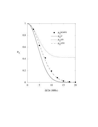
Figure 10: An example of an optical shielding study in a MOT from Ref. [66]. Shown is the shielding measure $P_{S}$ as the function of the Rabi frequency $\Omega$. $P_{S}$ describes the ground state population flux at very short range. The dots are results of the Monte Carlo simulations and the lines presents the results of various semiclassical Landau-Zener approaches (see text). When the laser field is strong enough, the ground state is effectively emptied before the atoms have a chance to approach close to each other. This is demonstrated by the decreasing value of $P_{S}$ for increasing Rabi frequencies.

In this Section we have described radiative heating and optical shielding processes by using the molecular state description. This is how the treatment has usually been done in the past when studying the heating and loss of atoms in MOTs. In our calculations and simulations we use the two-atom product state presentation instead. Our aim is to study the effect of collisions in a near-resonant optical lattice. Most of the photon scattering still occurs when the atoms are outside the range of a binary interaction. It would be an unnecessary complication to describe photon scattering and quantum jumps in a lattice by using a molecular basis. Moreover, we give a simultaneous description for laser cooling and collision processes. Hence, in our case the molecular basis is only used for a qualitative description of radiative heating and optical shielding processes, but it does not appear directly in our calculations.

4 Collisions in optical lattices

In the past cold binary collisions between atoms have been widely studied under conditions which correspond to the atoms trapped in magneto-optical traps [8, 9, 22]. Previous cold collision research has concentrated on the effects of inelastic collisions on the properties of an atomic cloud, but has neglected the co-existence of the cooling processes.

We are dealing with near-resonant optical lattices, and we have combined in a single framework the cooling and cold collision dynamics. Thus our approach includes simultaneous dynamical processes of cooling, trapping, and collisions in atom gas.

For far off-resonant lattices the possibility to control the cold collisions coherently has been proposed [71] and realized in an experiment [33]. This allows the creation of an entanglement between the atoms, a step towards quantum computing in optical lattices [72]. Moreover, the observation of superfluid–Mott-insulator phase transition helps in filling in the sites of the far-off resonant lattice by controlled particle number [5]. For dissipative optical lattices, the creation of a double optical lattice opens interesting prospect for cold collision studies in the presence of near-resonant light [34].

Radiative heating and optical shielding studies in MOTs typically use the molecular state description of the binary atomic system. After choosing the specific excited molecular state and doing the partial wave expansion, usually only the lowest relative angular momentum ground and excited state are accounted. The other option has been to consider independent pairs of partial wave states, neglecting the coupling between the pairs in a weak field approximation [65]. Thus the descriptions in the past have been two-state models, neglecting the multitude of internal states of the atoms, and without the position dependent coupling between the atoms and the laser field. For optical lattices the internal states of the atoms have to be accounted because of the spatial periodicity of the coupling caused by the polarization gradients of the laser field.

We use the two-atom product state basis [73]. For two six-level atoms in the red-detuned case this means $36$ basis states. If the basis is transformed into a molecular one, there are manifolds of attractive and repulsive molecular states buried in our description. We are forced to do the calculations in one dimension since the limited amount of computational resources. It is also worth noting that the simple atomic level schemes we consider, do not allow to account for the spatially dependent adiabatic couplings between the atomic states which play a role in the system dynamics for more complex level schemes [17].

A resonant dipole-dipole interaction between the atoms in optical lattices has been studied with nondynamic approaches [74, 75, 76, 77, 78]. Usually these studies assume fixed positions for the atoms and concentrate on the mean-field type descriptions of the lattice system. These approaches neglect the dynamical nature of the cold collisions, and the inelastic processes of radiative heating or incomplete optical shielding. Our approach includes the dynamical processes of cooling and cold collisions in the same framework. It is important to note that once the atoms are localized into the optical lattice sites, they are still able to move around in the lattice. For shallow lattices this is because the quantum-mechanical tunneling probability between the lattice sites is not negligible. For deep optical lattices, which are more relevant to our case, the atomic motion between the wells may be induced by the recoil effects combined with the optical pumping process.

For the lattice parameters we use, we have noticed that the inter-well effects are negligible and our interest lies in the case when two atoms end up in the same lattice site and collide. The intra-well collision partners may then gain kinetic energy due to an inelastic collision and escape from the lattice. In the case of optical shielding, the possibility of making the collisions elastic and preventing the atoms from close encounters would also prevent the atoms to escape from the lattice.

Numerical simulations are extremely heavy, especially in the case of red-detuned lattices where the level scheme can not be simplified. For the required computer resources, see Appendix A. We are forced to make some simplifications to our model, for details see [37]. Most importantly, we have to neglect the reabsorption of the scattered photons. With increasing atomic density, reabsorption may heat the atomic cloud and cause radiation pressure to outward direction from the trap center [10], limiting the achievable atomic densities. In the blue-detuned lattice, the number of scattered photons is largely reduced because the center of each lattice site corresponds to a completely dark point in space. For red-detuned lattices we merely describe the effects of collisions on the thermodynamical properties of the cloud. The full thermodynamics is not described since we neglect reabsorption. This poses some limitations for the applicability of our results in red-detuned lattices, but for the blue-detuned case our description is close to the complete thermodynamical description because the scattering is generally low.

In the following Subsection we describe how we calculate the interaction matrix elements between two multistate atoms, especially the resonant dipole-dipole interaction matrix elements. The whole problem is then formulated by using the MCWF method. For details, see Ref. [37]. The Section ends with the presentation of the central results.

4.1 Resonant dipole-dipole interaction

One of the early treatments for resonant dipole-dipole forces between two atoms was given already at the end of the 30’s [79], and the retardation effects were discussed almost a decade later [80]. Later on, Lenz and Meystre considered the resonant dipole-dipole interaction (DDI) for two two-level atoms in a standing-wave field [81]. Our derivation follows their approach and makes the generalization to the multilevel atom case.

The DDI is the first interaction to come into play when the colliding atoms approach each other in dissipative optical lattice. Since the interaction between the atoms is mediated by the quantized environment, the natural starting point is the two-atom system master equation and its damping part describing the coupling of the system to the electromagnetic environment [81] [see also Eq. (14)]

$$\dot{\rho} = -\frac{1}{\hbar^{2}}\int_{0}^{t}d\tau Tr_{f}\left\{H_{sf}(t)H_{sf}(\tau)\rho_{sf}(\tau)-H_{sf}(t)\rho_{sf}(\tau)H_{sf}(\tau)\right.$$ (15)

$$\left.-H_{sf}(\tau)\rho_{sf}(\tau)H_{sf}(t)+\rho_{sf}(\tau)H_{sf}(\tau)H_{sf}(t)\right\},$$

where $\rho$ is the reduced density matrix of the two-atom system, $\rho_{sf}$ the density matrix of the two-atom system and the field, $H_{sf}$ denotes the system-field interaction Hamiltonian, and $Tr_{f}$ the trace over the field.

We expand the electromagnetic field in the standard way

$${\bf E}({\bf r}_{\alpha}) = {\bf E}^{+}({\bf r}_{\alpha})+{\bf E}^{-}({\bf r}_{\alpha})$$

$${\bf E}^{+}({\bf r}_{\alpha}) = \sum_{\bf{k}}i{\cal E}({\bf k}){\bf a}_{\bf k}e^{i{\bf k\cdot{\bf r}_{\alpha}}}$$

$${\bf E}^{-}({\bf r}_{\alpha}) = \left({\bf E}^{+}({\bf r}_{\alpha})\right)^{{\dagger}},$$ (16)

where ${\bf a_{\bf k}}$ is the annihilation operator for mode ${\bf k}$, ${\bf r}_{\alpha}$ denotes the position of atom $\alpha$, and

$${\cal E}({\bf k})=\sqrt{\frac{2\pi\hbar\omega({\bf k})}{V}}{\bf\epsilon}_{j}({\bf k}),$$ (17)

where ${\bf\epsilon}_{j}$ is the polarization vector and $V$ the quantization volume.

We use the center of mass and relative coordinates of the atom pair

$${\bf R} = \frac{{\bf r}_{1}+{\bf r}_{2}}{2},~{}~{}{\bf r}={\bf r}_{2}-{\bf r}_{1},$$ (18)

and the notation

$$S_{+,q} = \sum_{m}CG_{m}^{q}\left(|e_{m+q}\rangle_{1}~{}_{1}\langle g_{m}|+|e_{m+q}\rangle_{2}~{}_{2}\langle g_{m}|\right)$$

$$\Delta S_{+,q} = \sum_{m}CG_{m}^{q}\left(|e_{m+q}\rangle_{1}~{}_{1}\langle g_{m}|-|e_{m+q}\rangle_{2}~{}_{2}\langle g_{m}|\right),$$ (19)

where $CG_{m}^{q}$ are the appropriate Clebsch-Gordan coefficients, $q$ is the polarization label in the spherical basis, and sub-indices label the two atoms. The interaction between the two-atom system and the vacuum electromagnetic field can now be written as

$$H_{sf} = i\sum_{{\bf k},{\bf\epsilon}_{j}}\sqrt{\frac{2\pi\hbar\omega({\bf k})}{V}}d\left\{\epsilon_{j,+}\left[\cos\left({\bf k}\cdot\frac{\bf r}{2}\right)S_{+,+}-i\sin\left({\bf k}\cdot\frac{\bf r}{2}\right)\Delta S_{+,+}\right]\right.$$ (20)

$$+\epsilon_{j,0}\left[\cos\left({\bf k}\cdot\frac{\bf r}{2}\right)S_{+,0}-i\sin\left({\bf k}\cdot\frac{\bf r}{2}\right)\Delta S_{+,0}\right]$$

$$\left.+\epsilon_{j,-}\left[\cos\left({\bf k}\cdot\frac{\bf r}{2}\right)S_{+,-}-i\sin\left({\bf k}\cdot\frac{\bf r}{2}\right)\Delta S_{+,-}\right]\right\}e^{i{\bf k}\cdot{\bf R}}e^{i\omega_{0}t}{\bf a}_{{\bf k},j}$$

$$+H.c.,$$

where $\epsilon_{j,q}$ is the projection $\epsilon_{j,q}={\bf\epsilon}_{j}\cdot{\bf\epsilon}_{q}$ on the spherical basis ${\bf\epsilon_{0}},{\bf\epsilon}_{\pm}$, and $d$ the dipole moment of the atomic transition.

One can identify the DDI interaction terms between the atoms as those having $\langle n_{\omega}+1\rangle=1$ where $n_{\omega}$ is the number of photons in the mode of the environment with mode frequency $\omega$. In another words, the average photon number in the interaction process is zero since the DDI interaction can be viewed as an exchange of excitation between the two atoms via the environment vacuum field. After lengthy analytical calculations following [81], and using the arguments from Ref. [82], one can write down the expression for the three-dimensional resonant dipole-dipole interaction as

$$V_{dip} = -\frac{3}{8}\hbar\Gamma\left\{\frac{1}{3}\frac{\cos q_{0}r}{q_{0}r}\left[1-2P_{2}(\cos\theta_{r})\right]\left({\cal S}_{++}{\cal S}_{-+}+{\cal S}_{+-}{\cal S}_{--}-2{\cal S}_{+0}{\cal S}_{-0}\right)\right.$$ (21)

$$-2\left[\frac{\sin q_{0}r}{(q_{0}r)^{2}}+\frac{\cos q_{0}r}{(q_{0}r)^{3}}\right]P_{2}(\cos\theta_{r})\left({\cal S}_{++}{\cal S}_{-+}+{\cal S}_{+-}{\cal S}_{--}-2{\cal S}_{+0}{\cal S}_{-0}\right)$$

$$+\frac{1}{3}\left[-\frac{\cos q_{0}r}{q_{0}r}+3\left(\frac{\sin q_{0}r}{(q_{0}r)^{2}}+\frac{\cos q_{0}r}{(q_{0}r)^{3}}\right)\right]\times$$

$$\left[\frac{1}{\sqrt{2}}P_{2}^{1}(\cos\theta_{r})\cos\phi_{r}\left(-{\cal S}_{++}{\cal S}_{-0}+{\cal S}_{+0}{\cal S}_{--}-{\cal S}_{+0}{\cal S}_{-+}+{\cal S}_{+-}{\cal S}_{-0}\right)\right.$$

$$+P_{2}^{2}(\cos\theta_{r})\cos 2\phi_{r}\left.\left.\left({\cal S}_{++}{\cal S}_{--}+{\cal S}_{+-}{\cal S}_{-+}\right)\frac{}{\!}\right]\right\},$$

where $q_{0}=\omega_{0}/c$, $P_{2}$ is Legendre polynomial, $P_{m}^{n}$ are the associated Legendre functions, and $\Gamma$ is the linewidth of the atomic excited state. The angles $\theta_{r}$ and $\phi_{r}$ are the angles of the relative coordinate ${\bf r}$ in the spherical basis. We have also introduced the operators

$${\cal S}_{+q}{\cal S}_{-q^{\prime}}\equiv\left(S_{+,q}^{1}S_{-,q^{\prime}}^{2}+S_{+,q}^{2}S_{-,q^{\prime}}^{1}\right),$$ (22)

where $S_{-,q}^{\alpha}=\left(S_{+,q}^{\alpha}\right)^{\dagger}$ and

$$S_{+,q}^{\alpha}=\sum_{m=-J_{g}}^{m=J_{g}}CG_{m}^{q}|e_{m+q}\rangle_{\alpha}~{}_{\alpha}\langle g_{m}|.$$ (23)

Here $\alpha$ labels one of the two atoms.

If the two atoms are positioned on the $z$-axis, the DDI potential reduces to the one-dimensional potential

$$V_{dip}^{axis} = \frac{3}{8}\hbar\Gamma\left\{\frac{1}{3}\frac{\cos q_{0}r}{q_{0}r}+2\left[\frac{\sin q_{0}r}{(q_{0}r)^{2}}+\frac{\cos q_{0}r}{(q_{0}r)^{3}}\right]\right\}\times$$ (24)

$$~{}~{}~{}\left({\cal S}_{++}{\cal S}_{-+}+{\cal S}_{+-}{\cal S}_{--}-2{\cal S}_{+0}{\cal S}_{-0}\right).$$

It is worth noting that the interaction potential (24) includes the retardation effects. By diagonalizing $V_{dip}$, it is possible to obtain the molecular potentials shown in Fig. 11. We use the molecular basis occasionally for the qualitative description of the collision processes and emphasize that the calculations are done in the two-atom product state basis.

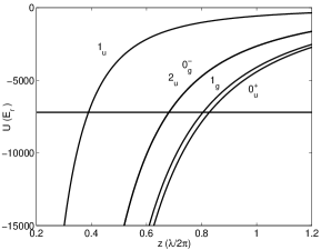
Figure 11: The energy shifted ground state and the attractive excited state [labeled by the Hund’s case (c) notation] molecular potentials of Cs₂ for $\delta=-3.0\Gamma$. The repulsive potential manifold is not shown.

4.2 Monte Carlo wave-function formulation

We use a variant of the Monte Carlo (MC) method which was developed by Dalibard, Castin, and Mølmer [45, 46, 47]. The core idea of the Monte Carlo wave-function (MCWF) method is the generation of a large number of single wave function realizations including stochastic quantum jumps of the system studied. Quantum jumps occur to the available decay channels of the system whose environment is continuously monitored. In our case, detection of a photon corresponds to a quantum jump from an internal excited electronic state to the ground electronic state of an atom in an optical lattice. Solutions for the steady state density matrix and system properties can be calculated as ensemble averages of single wave-function realizations.

In general, we look for the solution of the master equation (14) whose relaxation part is in the so called Lindblad form [83]

$${\cal L}_{rel}\left[\rho\right]=-\frac{1}{2}\sum_{i}\left(C_{i}^{{\dagger}}C_{i}\rho+\rho C_{i}^{{\dagger}}C_{i}\right)+\sum_{i}C_{i}\rho C_{i}^{{\dagger}},$$ (25)

where the summation over $i$ include the system operators $C_{i}$ and their adjoints $C_{i}^{{\dagger}}$ (we define these operators in a moment).

To unravel the appropriate master equation by generating the realizations for the MC ensemble, one solves the time dependent Schrödinger equation

$$i\hbar\frac{\partial|\psi\rangle}{\partial t}=H|\psi\rangle.$$ (26)

In our case $|\psi\rangle$ describes the time-dependent two atom wave-function in position space

$$|\psi(z_{2},t)\rangle=\sum_{j_{1},j_{2},m_{1},m_{2}}\psi^{j_{1},m_{1}}_{j_{2},m_{2}}(z_{2},t)|j_{1}{m_{1}}\rangle_{1}|j_{2}{m_{2}}\rangle_{2},$$ (27)

where $j_{1}$ and $j_{2}$ denote the ground and excited states of atom $1$ and $2$ respectively, $m_{1}$ and $m_{2}$ the $z$-component of the angular momentum. Due to the limited availability of computer resources we have to fix the position of atom 1 by setting $z_{1}=0$, and $z_{2}$ is then the both position of the moving atom 2 in the lattice, as well as the relative coordinate [37].

The non-Hermitian Hamiltonian $H$ in Eq. (26) is

$$H=H_{S}+H_{DEC},$$ (28)

where the system Hamiltonian $H_{S}$ in our case includes the atom-laser interaction Hamiltonians expanded in the two-atom Hilbert space, and the resonant dipole-dipole interaction between the atoms, Eqs. (7,10,24).

The non-Hermitian part includes the sum over the various allowed decay channels $j$,

$$H_{DEC}=-\frac{i\hbar}{2}\sum_{j}C_{j}^{\dagger}C_{j},$$ (29)

where $C_{j}$ are the jump operators corresponding to particular decay channels and can be found out from the relaxation part of the master equation (25).

During a discrete time evolution step of length $\delta t$ the norm of the wave function may shrink due to $H_{DEC}$. The amount of shrinking gives the probability of a quantum jump to occur during the short interval $\delta t$. Based on a random number one then decides whether a quantum jump occurred or not. Before the next time step is taken, the wave function of the system is renormalized. If and when a jump occurs, one performs a rearrangement of the wave function components according to the jump operator $C_{j}$, corresponding to the decay channel $j$, before renormalization of $|\psi\rangle$.

For example, if we denote the jump of atom 1 from $|e_{-1/2}\rangle_{1}$ to $|g_{-1/2}\rangle_{1}$ as channel 2 in our red-detuned lattice studies, the jump operator in the product state basis for this jump is

$$C_{2} = \sqrt{2/3}\sqrt{\Gamma}\left\{|g_{-1/2}\rangle_{1}~{}|g_{-1/2}\rangle_{2}~{}_{1}\langle e_{-1/2}|~{}_{2}\langle g_{-1/2}|\right.$$ (30)

$$+|g_{-1/2}\rangle_{1}~{}|g_{+1/2}\rangle_{2}~{}_{1}\langle e_{-1/2}|~{}_{2}\langle g_{+1/2}|$$

$$+|g_{-1/2}\rangle_{1}~{}|e_{-3/2}\rangle_{2}~{}_{1}\langle e_{-1/2}|~{}_{2}\langle e_{-3/2}|$$

$$+|g_{-1/2}\rangle_{1}~{}|e_{-1/2}\rangle_{2}~{}_{1}\langle e_{-1/2}|~{}_{2}\langle e_{-1/2}|$$

$$+|g_{-1/2}\rangle_{1}~{}|e_{+1/2}\rangle_{2}~{}_{1}\langle e_{-1/2}|~{}_{2}\langle e_{+1/2}|$$

$$\left.\!+|g_{-1/2}\rangle_{1}~{}|e_{+3/2}\rangle_{2}~{}_{1}\langle e_{-1/2}|~{}_{2}\langle e_{+3/2}|\right\}.$$

Here, the factor $\sqrt{2/3}$ is the Clebsch-Gordan coefficient of the corresponding transition. After applying the jump operator $C_{j}$, the wave function is still in a superposition state, but it has collapsed into a subspace of the product state basis vectors, leaving only one ground state level component of the atom populated.

In general, the jump probability into the decay channel $j$ for each of the time-evolution step $\delta t$ is

$$P_{j}=\delta t\langle\psi|C_{j}^{\dagger}C_{j}|\psi\rangle.$$ (31)

Thus, the jump probability for an example channel $2$ in Eq. (30) for each time step is

$$P_{2} = \frac{2}{3}\delta t\Gamma\left\{|\psi^{e_{-3/2}}_{g_{-1/2}}|^{2}+|\psi^{e_{-3/2}}_{g_{+1/2}}|^{2}+|\psi^{e_{-3/2}}_{e_{-3/2}}|^{2}\right.$$ (32)

$$+\left.|\psi^{e_{-3/2}}_{e_{-1/2}}|^{2}+|\psi^{e_{-3/2}}_{e_{+1/2}}|^{2}+|\psi^{e_{-3/2}}_{e_{+3/2}}|^{2}\right\}.$$

Reference [37] presents in detail the implementation of the MCWF method in our lattice studies. There is a large number of numerical problems one has to solve for the MC implementation of two atoms in a lattice, for a list and solutions see Ref. [37]. For general numerical tools, e.g. split Fourier or Crank-Nicholson methods, to solve time dependent Schrödinger equation, see Ref. [84].

4.3 Red-detuned lattices

In this Subsection we present the main results from Refs. [36, 37] which deal with collision dynamics in red-detuned lattices. The main collision process in this case is radiative heating, see Section 3.1.

Once the atoms are localized into the lattice sites, they are still able to move around in the lattice. When the occupation density of the lattice increases one can ask what is the effect of collisions for the cooling dynamics in optical lattices, and how the cold collisions affect the atomic cloud once the atoms are localized.

At the beginning of the efficient cooling period a large fraction of atoms have higher kinetic energy than the optical lattice modulation depth. Atoms then have a high mobility and change their internal state frequently via the optical pumping cycles which cool them. A priori one might assume that the possible consequence of collisions would be a slowing of the cooling process, heating, and escape of the atoms from the lattice. Radiative heating studies at low temperatures in MOTs show a smooth widening of the momentum probability distribution corresponding to heating for large range of parameters [64, 65], see Fig. 8. A similar effect might be expected to occur in an optical lattice as well.

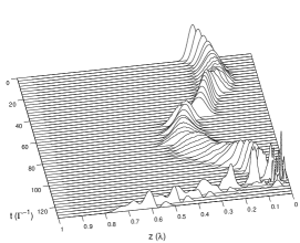
Figure 12: An example of a single wave packet realization from the full MC ensemble in position space (note the direction of $z$-axis because of the viewing angle). At the beginning of the time evolution the atom oscillates in the lattice well which has the center at $z=0.25\lambda$. It then approaches point $z=0$ (the position of the fixed atom), collides with another atom, and gains enough kinetic energy to be ejected from the lattice.

It turns out that the internal structure of the atoms and the spatial dependence of the atom-field coupling changes the consequences of the collisions to some extent. Lattice structure introduces selectivity into the collision processes and atomic dynamics. In a lattice, the mobility of an atom between the lattice sites depends essentially on the kinetic energy, especially once the atoms are localized into the lattice sites. An atom, which has a large oscillation amplitude (corresponding to a large kinetic energy) in the lattice site, has a higher probability to change its internal ground state by optical pumping than an atom which is tightly localized into the vicinity of the center of the potential well. Rich dynamical features of the wave packet, like breathing and oscillations in a single lattice site, arise due to the fact that the packet here describes a superposition of the populations in the vibrational states of a lattice potential [84].

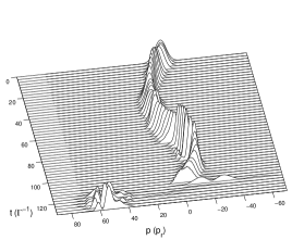
Figure 13: The same MC realization as in Fig. 12 but shown here in momentum space. The population is transferred to the high values of momentum due to the collision, and the atom consequently escapes from the lattice.

Since the high kinetic energy atoms are more mobile compared to their low kinetic energy partners, the high kinetic energy atoms have also a higher collision probability. During the same period of time the high-energy atoms change their internal ground state and the corresponding optical potential more often than tightly localized atoms. Thus, the coverage of various lattice sites, and the corresponding collision probability, is higher for more mobile atoms.

With these assumptions the consequence of collisions might be simple heating of the atomic cloud, or escape of the atoms from the lattice. The essential ingredient for a large kinetic energy increase is a high excitation probability of a quasimolecule. This depends on the curvature of the molecular potentials at a resonant Condon point and especially on the relative velocity between the colliding atoms. The optical lattice modulation depth defines the initial velocity distribution of the atoms when they start to move between the lattice sites after localization. It turns out that in a lattice, detuned a few atomic linewidths below the atomic resonance, and for lattice depths of a few hundred recoil energies, the surroundings are very favorable for strong excitation of the quasimolecule and the corresponding large kinetic energy changing collisions. The consequence is that the atoms mainly leave the lattice when colliding, and the total effect is the ejection of the hot atoms from the lattice. The ones which remain in a lattice have lower average kinetic energy per atom than in the low occupation density case of the lattice when there is no need to account for the interactions between the atoms. Figures 12 and 13 show in position and momentum spaces, respectively, an example of a collision which ejects the atoms from the lattice.

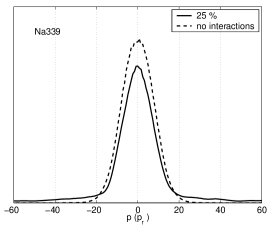
Figure 14: An example of momentum probability distributions for interacting and non–interacting atoms in a red-detuned optical lattice [37]. The momentum $p$ is expressed in the recoil unit $p_{r}=\hbar k_{r}$. For interacting atoms the distribution gets narrower compared to non-interacting atoms. The results correspond to a sodium lattice with lattice the depth $U_{0}=339E_{r}$, detuning $\delta=-3.0\Gamma$, and Rabi frequency $\Omega=2.8\Gamma$.

The selective escape mechanism resembles evaporative cooling used to produce BEC in magnetic traps. Here the rethermalization of the remaining atoms is more limited, though. Anyhow, spatial dependence of the laser field introduces selective heating of the hot atoms, and the consequent escape from the lattice. It would probably be too far reaching to claim that this effect should be visible in an experiment. Our model neglects the reabsorption of photons which may affect the total thermodynamics of the atomic cloud at high densities, and we neglect also the Doppler cooling. Thus we have revealed one aspect of the thermodynamics of a densely-populated near-resonant optical lattice but the solution for the complete problem is simply out of reach for the modern computational resources.

Figure 14 shows an example of the results for collisions in a red-detuned lattice from Ref. [37]. This example is for a sodium lattice of depth $U_{0}=339E_{r}$. The comparison is done between the momentum probability distributions of the interacting and non-interacting cases with the occupation density of $25\%$ of the lattice. The central peak is clearly narrower when the interactions between the atoms have been included. This central peak corresponds to the atoms which are trapped in a lattice, and the wide wings correspond to background atoms which are presumably out of the recapture range of the lattice and ejected from the lattice.

One can calculate by semi-classical means the excitation and survival probability for various molecular potentials. We have done a simple semi-classical analysis by using Landau-Zener approach in Ref. [37]. This analysis supports the conclusions presented above and shows the high probability for the atom pair to gain kinetic energy by the amount with which the collision partners are kicked out from the lattice.

4.4 Blue-detuned lattices

The prospect of using the trapping and cooling lasers for efficient optical shielding has been studied in Ref. [39]. Complete optical shielding would make collisions between atoms, when they end up in a same lattice site, elastic, and it would also prevent atoms from close encounters, reducing, e.g., inelastic hyperfine changing collisions. Thus efficient optical shielding could be beneficial in optical lattices in addition to the typical darkness of the blue-detuned lattices. The number of scattered photons in gray-lattices can be roughly two orders of magnitude smaller than in MOTs [40]. The role of the radiation pressure due to the reabsorption of photons diminishes, and our simplified model describes in a more realistic way the total thermodynamics of the atomic cloud, not only the collision aspect of the thermodynamics.

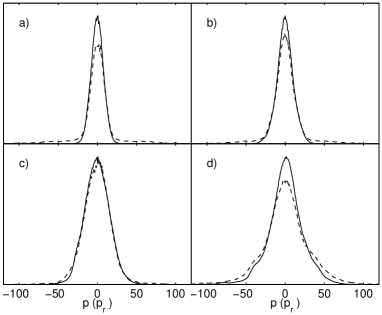
Figure 15: The momentum probability distributions for the $\delta=5\Gamma$ blue lattice case. The Rabi frequencies are: a) $\Omega=1.5\Gamma$, b) $\Omega=2.0\Gamma$, c) $\Omega=3.0\Gamma$, and d) $\Omega=5.0\Gamma$. The momentum $p$ is expressed in the recoil unit $p_{r}=\hbar k_{r}$. The dashed line is for the interacting and the solid line for the non–interacting atoms. When $\Omega$ increases the regime changes from incomplete shielding, a) and b), to complete shielding, c), and finally to off–resonant heating in d). The momentum distributions also get wider due to the deepening of the lattice with increasing $\Omega$.

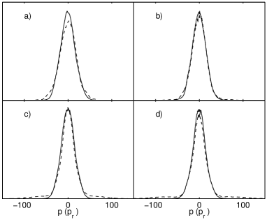
Figure 16: Momentum distributions for fixed $U_{0}\sim 710E_{r}$. a) $\delta=1.5\Gamma$ b) $\delta=5.0\Gamma$ c) $\delta=7.0\Gamma$ d) $\delta=10.0\Gamma$. The off-resonant processes play a role at the small detuning, a). In the intermediate detuning shielding may become complete and the collisions between atoms are elastic, b). For larger detuning the shielding is incomplete, c) and d).

Figure 15 presents the results of the simulations where the detuning is fixed to $\delta=5\Gamma$ [39]. The results show clearly how the efficiency of the shielding changes. When the coupling laser is weak, a large number of the collisions are still inelastic ones. Wide wings appear in the momentum probability distribution, see Figs. 15 (a) and 15 (b). All the population, which is excited at the Condon point, does not return to the ground state when the atoms move apart again. The quasimolecule slides down on the tail of the repulsive state producing a mild heating effect [66]. For a moderate field strength it is hard to see differences between the distributions for the interacting and non-interacting atoms, Fig. 15 (c). The optical shielding has become complete and atoms collide elastically when they end up in the same lattice site. The collision partners begin to move apart at large internuclear distances and also the short range unwanted effects are avoided. A further increase in the laser field strength makes it possible for the population to be excited into the attractive molecular state by off-resonant means [67]. This is the reason for the deviation of the two distributions in Fig. 15 (d), where the appearance of the wings is also qualitatively different than in the weak-field case of incomplete shielding.

Figure 16 presents another view to the shielding studies [39]. Instead of keeping the laser detuning fixed, here the lattice modulation depth is kept nearly constant. It turns out that for a very small detuning, Fig. 16 (a), the off-resonant effects heat the atomic cloud. This corresponds to the regime where $\Omega/\delta>1$, and the steady state formation between the ground and the excited states surpasses the dynamical resonant excitation process. When the detuning is increased, the point of complete shielding is reached, Fig. 16 (b). In the region where $\Omega/\delta\ll 1$, Fig. 16 (c) and (d), shielding becomes incomplete again due to the weak excitation and stimulated re-excitation in Condon point.

The results demonstrate clearly that the co-existence of cooling, trapping, and shielding processes is possible in blue-detuned near-resonant optical lattices. The shielding is not always complete but by the careful choice of parameters shielding becomes very efficient. Moreover, this can be obtained within a typical and convenient parameter regime for near-resonant lattices, e.g., in Fig. 15 (c) $\delta=5\Gamma$, $\Omega=3\Gamma$, and $U_{0}=712E_{r}$. A clear advantage here is the achievement of complete shielding with the same lasers which provide the cooling and trapping. This is in contrast to MOTs where one needs to introduce additional lasers for shielding.

Even though the available occupation densities in near-resonant optical lattices have been very low so far, the metastable rare-gas atoms could provide a convenient case for an experimental study of shielding in optical lattices due to the clear ion signal that marks collision events [85, 86].

The experimental work on optical shielding in MOTs show the saturation of the shielding phenomena when the intensity of the laser field is increased [9]. The saturation has not been present in earlier theoretical studies of shielding [66, 67], and we do not see the saturation of shielding here either. The results presented in Ref. [39] seem to confirm the view that the saturation does not arise due to spontaneous emission effects [66]. The reason for the saturation of shielding is still unclear. It has been attributed to various processes, in addition to the above-mentioned premature termination of shielding via spontaneous emission [66]. Other possibilities include counterintuitive or off-resonant processes involving different partial waves, or other processes that similarly involve multiple states (in contrast to the basic two-state approaches [9, 68, 87, 88]). In the case when several partial waves are considered, a net of Condon points (instead of only one resonant point of two-level models) opens a door for complicated excitation and de-excitation patterns which may affect the system dynamics [89]. The partial wave description is a useful frame of reference in normal collision studies to allow for more than one dimension. Due to the low collision velocities one can limit the studies to a few waves only. But the presence of an optical lattice forces us to abandon this description. Since our model is, due to the computational limitations, only one-dimensional, we can not conclusively that saturation of shielding should be absent in a lattice experiment.

So far there has been very few cold collision experiments in optical lattices [90, 91]. These experiments showed how the lattice structure affects the transport of atoms by using collisions as a probe. We hope that our work serves as a motivation for experimentalists to do shielding studies in blue-detuned optical lattices.

4.5 Collision rates

The results of Refs. [36, 37] show that in our selected parameter regime, i.e., the parameter regime for near-resonant lattices, the motion of the atom between the lattice sites (or in the lattice site occupied by the single atom only) is not strongly affected by other atoms, not at least for the occupation densities which we have used (maximum $25\%$). Hence, binary interactions between the atoms come into play only when two atoms simultaneously occupy the same lattice site. This makes it possible to develop a method to calculate the average rate at which two atoms end up in the same site, and the consequent cold collision rate in a lattice, by following the trajectories of single atoms [38]. Cold collision rate refers here to the average rate of atoms to reach the region of the resonant Condon point in the presence of near-resonant light and describes the rate of occurrence of radiative heating events in a red-detuned lattice, or optical shielding events, if blue-detuned light is used. It is assumed that the two atoms always collide when they end up in the same lattice site. For the parameters used here, this assumption is confirmed by the results in Refs. [36, 37].

The basic idea of the developed method is as follows. A possible trajectory of an atom in optical lattice is given by a single MCWF realization. Trajectories in position space can then give information about the rate at which atoms travel over the average distance $z_{a}$ between the atoms, which in turn gives information about the binary collision rate in a lattice. The average distance between atoms $z_{a}$ corresponds to the mean free path of atoms between collision events in our one-dimensional model. Thus, if we monitor the transport of atoms in the lattice over the average distance between the atoms, or the atomic flux over the average distance, we also obtain information about the collision rates.

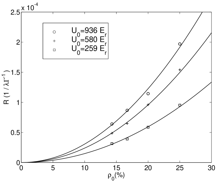
Figure 17: The binary collision rate $R$ for three different lattice depths $U_{0}$ as a function of occupation density $\rho_{0}$ of the lattice [38]. The points show the simulation results, and the solid lines the quadratic collision rate curves averaged from the simulation results for the specific red-detuned lattice. The detuning is kept constant at $\delta=-3.0\Gamma$ whereas the Rabi frequency increases as $\Omega=1.0\Gamma,1.5\Gamma,1.9\Gamma$ with the increasing lattice depth indicated in the legend.

Figure 17 displays the calculated collision rates as a function of the occupation density of the lattice for three different lattice depths [38]. In our simple 1D case the collision rate does not depend on the scattering cross section and collisions are a measure of transport in a lattice. This was also the case in the experimental study of Ref. [91]. In both cases the collision rate has a quadratic behavior.

The points in Fig. 17 are the simulation results and the solid lines quadratic fits. It is interesting to note from the Monte Carlo point of view that we get results for a wide density range by doing simulations for only a very few values of density. The possibility of obtaining the result for all the values of the variable, in this case occupation density, from single Monte Carlo ensemble is a new feature in the MCWF simulations to our knowledge, at least when the MCWF method is applied to cold collision problems.

Two-atom collision simulations in a lattice described in previous Subsections are computationally very heavy. It would be useful to find more simple means to do collision studies in optical lattices. The method presented above presents a step in this direction. For example, if the semiclassical analysis shows that for particular parameter values the colliding atoms have a high probability to be ejected from the lattice due to radiative heating, then the collision rate described here gives directly the loss rate of atoms from the lattice. MCWF simulations for one atom, like the ones reported in Ref. [38], are fairly simple and fast to perform. This is especially true when compared to the two-atom case. Thus the combination of these simple one-atom simulations with semiclassical models for intra-well collision effects have a potential to simplify the studies of binary collisions in optical lattices.

5 Conclusions

We have studied the cold collision dynamics between atoms in near-resonant, dissipative red- and blue-detuned optical lattices. The applied methods have been mainly based on the Monte Carlo wave-function method. A semiclassical analysis has been done which supports the conclusions drawn from the full quantum-mechanical calculations [37].

The implementation of the MCWF method to study cold collisions in optical lattices is not straightforward and the simulations have been very demanding from the computer resource point of view. This is due to the internal structure of atoms, coupling to the electromagnetic environment, position dependent coupling of the atoms to the laser field, and position dependent coupling between the atoms.

The results for near-resonant red-detuned lattices are in quite a sharp contrast to the interaction studies in magneto-optical traps. Instead of a heating, a cooling due to the selection of collision partners from high kinetic energy atoms is seen in the simulation results. The blue-lattice results show the applicability of optical shielding. Future collision studies require simplifications, for which we propose a simple way to calculate the collision rate in optical lattices.

In the past there has been many studies of cold collisions in magneto-optical traps, see the review [9]. The work presented in here extends the regime of cold collision studies into the realm of optical lattices. This is far from being a trivial step. The major reason is that for sub-Doppler cooling mechanisms, which exploit various polarization states of a laser field, it is necessary to account for the internal structure of atoms, and this greatly complicates the total system under study and the calculations. Moreover, it is not enough to formulate the problem using only the relative motion between the atoms in a constant laser field. The position of the atoms with respect to a lattice structure has to be accounted also.

In conclusion, we have shown how research on cold collisions in the present of near-resonant light can be extended from magneto-optical traps to cover also optical lattices. In future, the recently developed double optical lattice [34] opens interesting prospects for the experimental study on cold collisions in dissipative optical lattices.

Appendix A Required computational resources

The numerical simulations are demanding since we are dealing with a 36 level quantum system including various position dependent couplings and a dissipative coupling to the environment. We have used 32 processors of an SGI Origin 2000 machine, which has 128 MIPS R12000 processors of 1 GB memory per processor [92]. The total memory taken by a single simulation (fixed $\delta$, $\Omega$, occupation density $\rho_{o}$, and atomic species) is 14 GB, and generating a single history requires 6 hours of CPU time in red-detuned lattice studies. A simulation of 128 ensemble members then requires a total CPU time which is roughly equal to one month. The normal clock time is, of course, much shorter (roughly 22 hours) since we take advantage of powerful parallel processing for which the MCWF simulations suit very well.

References

- [1] Nichols E F and Hull G F 1901 Phys. Rev. 13 307
- [2] Chu S, Bjorkholm J E, Ashkin A, and Cable A 1986 Phys. Rev. Lett. 57 314
- [3] Anderson M H, Ensher J R, Matthews M R, Wieman C E, and Cornell E 1995 Science 269 198
- [4] DeMarco B and Jin D S 1999 Science 285 1703
- [5] Greiner M, Mandel O, Esslinger T, Hänsch T W, and Bloch I 2002 Nature 415 39
- [6] Greiner M, Regal C S, and Jin D S 2003 Nature 426 537; Jochim S, Bartenstein M, Altmeyer A, Hendl G, Riedl S, Chin C, Hecker Denschlag J, and Grimm R 2003 Science 302 2101; Zwierlein M W, Stan C A, Schunck C H, Raupach S M F, Gupta S, Hadzibabic Z, and Ketterle W 2003 Phys. Rev. Lett. 91 250401
- [7] Chin C, Bartenstein A, Altmeyer A, Riedl S, Jochim S, Hecker Denschlag J, and Grimm R 2004 Science 305 1128; Kinnunen J, Rodriguez M, and Törmä P 2004 Science 305 1131
- [8] Suominen K-A 1996 J. Phys. B 29 5981
- [9] Weiner J, Bagnato V S, Zilio S, and Julienne P S 1999 Rev. Mod. Phys. 71 1
- [10] Metcalf H J and van der Straten P 1999 Laser Cooling and Trapping (New York: Springer)
- [11] Stenholm S 1986 Rev. Mod. Phys. 58 699
- [12] Jessen P S and Deutsch I H 1996 Adv. At. Mol. Opt. Phys. 37 95
- [13] Adams C S and Riis E 1997 Prog. Quant. Electr. 21 1
- [14] Meacher D R 1998 Contemp. Phys. 39 329
- [15] Rolston S 1998 Phys. World 11(10) 27
- [16] Guidoni L and Verkerk P 1999 J. Opt. B 1 R23
- [17] Grynberg G and Robilliard C 2001 Phys. Rep. 355 335
- [18] Bloch I 2004 Phys. World 17(4) 25
- [19] Cohen-Tannoudji C 1992 Proc. of the Int. School of Physics Enrico Fermi, Course CXVIII - Laser Manipulation of Atoms and Ions (Varenna) Eds: Arimondo E et al(Amsterdam: Elsevier Science Publishers B.V.) p. 99
- [20] Grynberg G and Triché C 1996 Proc. of the Int. School of Physics Enrico Fermi, Course CXXXI - Coherent and Collective Interactions of Particles and Radiation Beams (Varenna) Eds: Aspect A et al(Amsterdam: IOS Press) p. 243
- [21] Hemmerich A, Weidemüller M, and Hänsch T W 1996 Proc. of the Int. School of Physics Enrico Fermi, Course CXXXI - Coherent and Collective Interactions of Particles and Radiation Beams (Varenna) Eds: Aspect A et al(Amsterdam: IOS Press) p. 503
- [22] Burnett K, Julienne P, Lett P, and Suominen K-A 1995 Phys. World 8 (10) 42
- [23] Dalibard J and Cohen-Tannoudji C 1989 J. Opt. Soc. Am. B 6 2023
- [24] Ungar P J, Weiss D S, Riis E, and Chu S 1989 J. Opt. Soc. Am. B 6 2058
- [25] Letokhov V L 1968 JETP Lett. 7 272
- [26] Burns M M, Fournier J-M, and Golovchenko J A 1990 Science 249 749
- [27] Birkl G, Gatzke M, Deutsch I H, Rolston S L, and Phillips W D 1995 Phys. Rev. Lett. 75 2823
- [28] Weidemüller M, Hemmerich A, Görlitz A, Esslinger T, and Hänsch T W 1995 Phys. Rev. Lett. 75 4583
- [29] Ben Dahan M, Peik E, Castin Y, and Salomon C 1996 Phys. Rev. Lett. 76 4508
- [30] Wilkinson S R, Bharucha C F, Madison K W, Niu Q, and Raizen M G 1996 Phys. Rev. Lett. 76 4512
- [31] Fischer M C, Gutiérrez-Medina B, and Raizen M G 2001 Phys. Rev. Lett. 87 040402
- [32] Hensinger W K, Häffner H, Browaeys A, Heckenberg N R, Helmerson K, McKenzie C, Milburn G J, Phillips W D, Rolston S L, Rubinsztein-Dunlop H, and Upcroft B 2001 Nature 412 52
- [33] Mandel O, Greiner M, Widera A, Rom T, Hänsch T W, and Bloch I 2003 Nature 425 937
- [34] Ellmann H, Jersblad J, and Kastberg A 2003 Phys. Rev. Lett. 90 053001
- [35] Castin Y, Dalibard J, and Cohen-Tannoudji C 1991 Proc. of Light Induced Kinetic Effects on Atoms, Ion and Molecules (Elba) Eds: Moi L et al(Pisa: ETS Editrice)
- [36] Piilo J, Suominen K-A, and Berg-Sørensen K 2001 J. Phys. B 34 L231
- [37] Piilo J, Suominen K-A, and Berg-Sørensen K 2002 Phys. Rev. A 65 033411
- [38] Piilo J 2003 J. Opt. Soc. Am. B 20 1135
- [39] Piilo J and Suominen K-A 2002 Phys. Rev. A 66 013401
- [40] Hemmerich A, Weidemüller M, Esslinger T, Zimmermann C, and T. Hänsch 1995 Phys. Rev. Lett. 75 37
- [41] Grynberg G and Courtois J-Y 1994 Europhys. Lett. 27 41
- [42] Petsas K I, Courtois J-Y, and Grynberg G 1996 Phys. Rev. A 53 2533
- [43] Esslinger T, Sander F, Hemmerich A, Hänsch T W, Ritsch H, and Weidemuller M 1996 Opt. Lett. 21 991
- [44] Stecher H, Ritsch H, Zoller P, Sander F, Esslinger T, and Hänsch T W 1997 Phys. Rev. A 55 545
- [45] Dalibard J, Castin Y, and Mølmer K 1992 Phys. Rev. Lett. 68 580
- [46] Mølmer K, Castin Y, and Dalibard J 1993 J. Opt. Soc. Am. B 10 524
- [47] Mølmer K and Castin Y 1996 Quantum Semiclass. Opt. 8 49
- [48] Plenio M B and Knight P L 1998 Rev. Mod. Phys. 70 101
- [49] Berg-Sørensen K, Castin Y, Mølmer K, and Dalibard J 1993 Europhys. Lett. 22 663
- [50] Castin Y and Mølmer K 1995 Phys. Rev. Lett. 74 3772
- [51] Castin Y and Dalibard J 1991 Europhys. Lett. 14 761
- [52] Marte P, Dum R, Taïeb R, Lett P D, and Zoller P 1993 Phys. Rev. Lett. 71 1335
- [53] Badescu S C, Ying S C, and Ala-Nissilä T 2001 Phys. Rev. Lett. 86 5092
- [54] Suominen K-A, Band Y B, Tuvi I, Burnett K, and Julienne P S 1998 Phys. Rev. A 57 3724
- [55] Petsas K I, Grynberg G, and Courtois J-Y 1999 Eur. Phys. J. D 6 29
- [56] Jersblad J, Ellmann H, Sanchez-Palencia L, and Kastberg A 2003 Eur. Phys. J. D 22 333
- [57] Greenwood W, Pax P, Meystre P 1997 Phys. Rev. A 56 2109
- [58] Movre M and Pichler G 1977 J. Phys. B 10 2631
- [59] Julienne P S and Vigué J 1991 Phys. Rev. A 44 4464
- [60] Drummond P D, Kheruntsyan K V, and He H 1998 Phys. Rev. Lett. 81 3055
- [61] Javanainen J and Mackie M 1999 Phys. Rev. A 59 R3186
- [62] Wynar R, Freeland R S, Han D C, Ryu C, and Heinzen D J 2000 Science 287 1016
- [63] Kos̆trun M, Mackie M, Côté R, and Javanainen J 2000 Phys. Rev. A 62 063616
- [64] Holland M J, Suominen K-A, and Burnett K 1994 Phys. Rev. Lett. 72 2367
- [65] Holland M J, Suominen K-A, and Burnett K 1994 Phys. Rev. A 50 1513
- [66] Suominen K-A, Holland M J, Burnett K, and Julienne P S 1995 Phys. Rev. A 51 1446
- [67] Suominen K-A, Burnett K, and Julienne P S 1996 Phys. Rev. A 53 R1120
- [68] Suominen K-A, Burnett K, Julienne P S, Walhout M, Sterr U, Orzel C, Hoogerland M, and Rolston S L 1996 Phys. Rev. A 53 1678
- [69] Landau L D 1932 Phys. Z. Sowjetunion 2 46
- [70] Zener C 1932 Proc. R. Soc. London Ser. A 137 696
- [71] Jaksch D, Briegel H-J, Cirac J I, Gardiner C W, Zoller P 1999 Phys. Rev. Lett. 82 1975
- [72] Jaksch D 2004 Contemp. Phys. 45 367
- [73] Cohen-Tannoudji C, Diu B, and Laloë F 1977 Quantum Mechanics Vol. I (Paris: Wiley-Interscience)
- [74] Goldstein E V, Pax P, and Meystre P 1996 Phys. Rev. A 53 2604
- [75] Boisseau C and Vigué J 1996 Opt. Commun. 127 251
- [76] Guzmán A M and Meystre P 1998 Phys. Rev. A 57 1139
- [77] Menotti C, and Ritsch H 1999 Phys. Rev. A 60 R2653
- [78] Menotti C, and Ritsch H 1999 Appl. Phys. B 69 311
- [79] King G W and van Vleck J H 1939 Phys. Rev. 55 1165
- [80] Casimir H B G and Polder D 1948 Phys. Rev. 73 360
- [81] Lenz G and Meystre P 1993 Phys. Rev. A 48 3365
- [82] Berman P R 1997 Phys. Rev. A 55 4466
- [83] Lindblad G 1976 Commun. Math. Phys. 48 119
- [84] Garraway B M and Suominen K-A 1995 Rep. Prog. Phys. 58 365
- [85] Katori H and Shimizu F 1994 Phys. Rev. Lett. 73 2555
- [86] Walhout M, Sterr U, Orzel C, Hoogerland M, and Rolston S L Phys. Rev. Lett. 74 506
- [87] Yurovsky V A and Ben-Reuven A 1997 Phys. Rev. A 55 3772
- [88] Napolitano R, Weiner J, and Julienne P S 1997 Phys. Rev. A 55 1191
- [89] Piilo J, Lundh E, and Suominen K-A 2004 Phys. Rev. A 70 013410
- [90] Kunugita H, Ido T, and Shimizu F 1997 Phys. Rev. Lett. 79 621
- [91] Lawall J, Orzel C, and Rolston S L 1998 Phys. Rev. Lett. 80 480
- [92] See CSC, the Finnish IT Center for Science, webpage www.csc.fi for details.