Theoretical and numerical investigation of the shock formation of dust ion acoustic waves

Abstract

We present a theoretical and numerical study of the self-steepening and shock formation of large-amplitude dust ion-acoustic waves (DIAWs) in dusty plasmas. We compare the non-dispersive two fluid model, which predicts the formation of large amplitude compressive and rarefactive dust ion-acoustic (DIA) shocks, with Vlasov/fluid simulations where ions are treated kinetically while a Boltzmann distribution is assumed for the electrons.

Shukla and Silin r1 predicted the existence of small amplitude dust ion-acoustic waves (DIAWs) in an unmagnetized dusty plasma. In the DIAWs, the restoring force comes from the pressure of inertialess electrons, while the ion mass provides the inertia to support the waves. On the timescale of the DIAWs, charged dust grains remain immobile, and they affect the overall quasi-neutrality of the plasma. When the dust grains are charged negatively, one has the depletion of the electrons in the background plasma. Subsequently, the phase speed [$\omega/k=(n_{i0}/n_{e0}+3T_{i}/T_{e})^{1/2}C_{s}$, where $n_{i0}$ $(n_{e0})$ is the unperturbed ion (electron) number density, $T_{i}$ $(T_{e})$ is the ion (electron) temperature, $C_{s}=(T_{e}/m_{i})^{1/2}$ is the ion acoustic speed, and $m_{i}$ is the ion mass] of the DIAWs becomes larger than the usual ion-acoustic speed in an electron-ion plasma without negatively charged dust, since $n_{i0}>n_{e0}$. When $n_{i0}\gg n_{e0}$ or $T_{i}\gg T_{e}$, small-amplitude DIAWs do not suffer Landau damping in a plasma, since the increased phase speed is much larger than the ion thermal speed $(T_{i}/m_{i})^{1/2}$. Small-amplitude DIAWs have been observed in laboratory experiments r2 , and the observed phase speed is in an excellent agreement with the theoretical prediction of Ref. r1 .

Recently, laboratory experiments r3 ; r4 ; r5 ; r6 have been conducted to study the formation of dust ion-acoustic (DIA) shocks in dusty plasmas. Dust ion acoustic compressional pulses have been observed to steepen as they travel through a plasma containing negatively charged dust grains. Theoretical models r7 ; r8 have been proposed to explain the formation of small amplitude DIA shocks in terms of the Korteweg-de Vries-Burgers equation, in which the dissipative terms comes from the dust charge perturbations r9 . Popel et al. r10 have included sources and sinks in the ion continuity equation, linear ion pressure gradients in the nonlinear ion momentum equation with a model collision term, as well as the dust grain charging equation to study the formation DIA shock-wave structures.

In this Brief Communication, we present analytical and numerical studies of large amplitude DIA shock waves in an unmagnetized dusty plasma PoP . We use fully nonlinear continuity and momentum equations for the warm ion fluid, as well as Boltzmann distributed electrons and the quasi-neutrality condition to examine the spatio-temporal evolution of large amplitude dust ion-acoustic pulses. We find simple-wave solutions of our fully nonlinear two fluid model, and compare them with those deduced from the time-dependent Vlasov simulations which uses initial conditions corresponding to the ones obtained from our theoretical model.

We consider an unmagnetized dusty plasma whose constituents are singly charged positive ions, electrons and charged dust grains. Thus, at equilibrium, we have $n_{i0}=n_{e0}-\epsilon Z_{d}n_{d0}$, where $\epsilon$ equals $-1$ $(+1)$ for negatively (positively) charged dust grains, $Z_{d}$ is the number of elementary charges residing on the dust grain, and $n_{d0}$ is the equilibrium dust number density. On the timescale of our interest, the dust grains are assumed to be immobile. The dynamics of low phase speed (in comparison with the electron thermal speed) nonlinear, dust ion-acoustic waves is governed by a Boltzmann distribution for the electrons

$$n_{e}=n_{e0}\exp\left(\frac{e\phi}{T_{e}}\right),$$ (1)

and the continuity and momentum equations for the ions

$$\frac{\partial n_{i}}{\partial t}+\frac{\partial(n_{i}v_{i})}{\partial x}=0,$$ (2)

and

$$\frac{\partial v_{i}}{\partial t}+v_{i}\frac{\partial v_{i}}{\partial x}=-\frac{e}{m_{i}}\frac{\partial\phi}{\partial x}-\frac{3T_{i}n_{i}}{m_{i}n_{i0}^{2}}\frac{\partial n_{i}}{\partial x},$$ (3)

where $n_{e}$ $(n_{i})$ is the total electron (ion) number density, $e$ is the magnitude of the electron charge, $\phi$ is the wave potential, and $v_{i}$ is the ion fluid velocity. The system is closed by means of Poisson’s equation

$$\frac{\partial^{2}\phi}{\partial x^{2}}=4\pi e(n_{e}-n_{i}-\epsilon Z_{d}n_{d0}).$$ (4)

In the following, we consider non-dispersive DIAWs, and use the quasi-neutrality condition $n_{e}=n_{i}+\epsilon Z_{d}n_{d0}$ instead of Eq. (4), together with the normalized variables $N=n_{i}/n_{i0}$, $u=v_{i}/C_{s}$, $\varphi=e\phi/T_{e}$, $z=r_{D}^{-1}x$ and $\tau=\omega_{pi}t$, where $\omega_{pi}=(4\pi n_{i0}e^{2}/m_{i})^{1/2}$ is the ion plasma frequency and $r_{D}=C_{s}/\omega_{pi}$ is the electron Debye radius. Thus, the system of equations (1)-(3) can be rewritten as

$$\frac{\partial u}{\partial\tau}+u\frac{\partial u}{\partial z}+\left(\frac{1}{N+\alpha-1}+3\eta N\right)\frac{\partial N}{\partial z}=0,$$ (5)

and

$$\frac{\partial N}{\partial\tau}+N\frac{\partial u}{\partial z}+u\frac{\partial N}{\partial z}=0,$$ (6)

where $\alpha=n_{e0}/n_{i0}$ and $\eta=T_{i0}/T_{e}$. In obtaining Eq. (5), we have used $\varphi=\mathrm{ln}[(N+\alpha-1)/\alpha]$ which follows from Eq. (1) and the quasineutrality condition.

In order to study the nonlinear evolution of large amplitude DIAWs, we seek simple wave solutions r11 of Eqs. (5) and (6). For this purpose, we rewrite them in the matrix form as

$$\frac{\partial}{\partial\tau}\left[\begin{matrix}u\\ N\end{matrix}\right]+\left[\begin{matrix}u&\frac{1}{N+\alpha-1}+3\eta N\\ N&u\end{matrix}\right]\frac{\partial}{\partial z}\left[\begin{matrix}u\\ N\end{matrix}\right]=\left[\begin{matrix}0\\ 0\end{matrix}\right].$$ (7)

Here, the nonlinear wave speeds are given by the eigenvalues

$$\lambda_{\pm}=u\pm N^{1/2}\left(\frac{1}{N+\alpha-1}+3\eta N\right)^{1/2}$$ (8)

of the square matrix multiplying the second term in Eq. (7). The square matrix in Eq. (7), which we denote $A$, can be diagonalized by a diagonalizing matrix $C$ whose columns are the eigenvectors of $A$, so that

$$C^{-1}AC=\Lambda\equiv\left[\begin{matrix}\lambda_{+}&0\\ 0&\lambda_{-}\end{matrix}\right],$$ (9)

where

$$C=\left[\begin{matrix}1&1\\ \left(\frac{1}{N(N+\alpha-1)}+3\eta\right)^{-1/2}&-\left(\frac{1}{N(N+\alpha-1)}+3\eta\right)^{-1/2}\end{matrix}\right],$$ (10)

and

$$C^{-1}=\left[\begin{matrix}\frac{1}{2}&\frac{1}{2}\left(\frac{1}{N(N+\alpha-1)}+3\eta\right)^{1/2}\\ \frac{1}{2}&-\frac{1}{2}\left(\frac{1}{N(N+\alpha-1)}+3\eta\right)^{1/2}\end{matrix}\right].$$ (11)

Multiplying Eq. (7) by $C^{-1}$ from the left gives the diagonalized system of equations

$$\frac{\partial\psi_{+}}{\partial\tau}+\lambda_{+}\frac{\partial\psi_{+}}{\partial z}=0,$$ (12)

and

$$\frac{\partial\psi_{-}}{\partial\tau}+\lambda_{-}\frac{\partial\psi_{-}}{\partial z}=0,$$ (13)

where the new variables are

$$\psi_{\pm}=\frac{u}{2}\pm\frac{1}{2}\int_{1}^{N}\left(\frac{1}{N^{\prime}(N^{\prime}+\alpha-1)}+3\eta\right)^{1/2}\,dN^{\prime}.$$ (14)

Equations (12) and (13) describe the DIAWs propagating in the positive and negative $z$ directions, respectively. Setting $\psi_{-}$ to zero, we have

$$u(N)=\int_{1}^{N}[1/N^{\prime}(N^{\prime}+\alpha-1)+3\eta]^{1/2}\,dN^{\prime},$$ (15)

which inserted into Eq. (12) gives

$$\lambda_{+}(N)=\int_{1}^{N}\left(\frac{1}{N^{\prime}(N^{\prime}+\alpha-1)}+3\eta\right)^{1/2}\,dN^{\prime}+N^{1/2}\left(\frac{1}{N+\alpha-1}+3\eta N\right)^{1/2}.$$ (16)

Since $\psi_{+}$ can be written as a function of $N$, Eq. (12) holds also for $N$, i.e.

$$\frac{\partial N}{\partial\tau}+\lambda_{+}(N)\frac{\partial N}{\partial z}=0,$$ (17)

which, as long as $N$ is continuous, has the general solution $N=f_{0}(\xi)$, where $\xi=x-\lambda_{+}(N)t$ and $f_{0}$ is the initial condition for $N$. We have plotted $\lambda_{+}$ as a function of $N$ in Fig. 1.

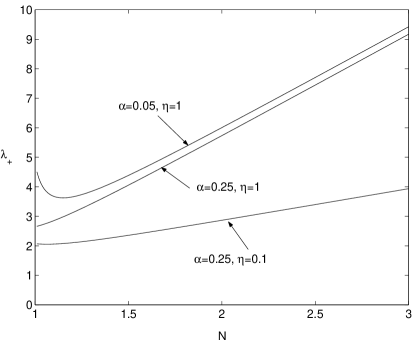
Figure 1: The wave speed $\lambda_{+}$ as a function of $N$ for different values on $\eta$ and $\alpha$.

Here, we see that $\lambda_{+}$ grows with increasing $N$ in the two cases with $\alpha=0.25$. In the case with $\lambda=0.05$, however, the phase speed first decreases for $N\approx 1$ before increasing with increasing $N$. In the small-amplitude limit, viz. $N=1+N_{1}$, where $|N_{1}|<<1$, we have the first-order Taylor expansion $\lambda_{+}=c+\gamma N_{1}$, where $c=(1/\alpha+3\eta)^{1/2}$ is the linear acoustic speed and $\gamma=(3\alpha+12\eta\alpha^{2}-1)/2\alpha(\alpha+3\eta\alpha^{2})^{1/2}$ is the coefficient in front of the nonlinear term. We note that $\gamma$ is negative for sufficiently small $\alpha$ (in agreement with the $\alpha=0.05$ case displayed in Fig. 1), and in the cold ion limit ($\eta=0$) we recover the result that $\alpha<1/3$ leads to a negative coefficient r8 ; r12 in front of the nonlinear term. The linear acoustic speed increases when $\alpha$ decreases. Thus, in the presence of negatively charged dust, the phase speed of the waves may becomes much larger than the ion acoustic speed, so that the Landau damping of the waves decreases r1 .

In order to compare the fluid and kinetic theories, we have solved the coupled Eqs. (5) and (6) numerically and compared the results with numerical solutions of the Vlasov equation. As an initial condition for our fluid simulations, we take a large-amplitude localized density pulse, $N=1.5-0.5\mathrm{sech}[3\sin(2\pi z/20000)+1.5]$, while the initial condition for the velocity is obtained from the simple wave solution as $u(N)=\int_{1}^{N}[1/N^{\prime}(N^{\prime}+\alpha-1)+3\eta]^{1/2}\,dN^{\prime}$. The results are compared with numerical solutions of the ion Vlasov equation

$$\frac{\partial f}{\partial\tau}+v\frac{\partial f}{\partial z}+\frac{\partial\varphi}{\partial z}\frac{\partial f}{\partial v}=0,$$ (18)

where $v$ has been normalized by $C_{s}$ and the ion distribution function $f$ by $n_{i0}/C_{s}$. Here, we have also used the quasineutrality condition and thus $\varphi=\mathrm{ln}[(N+\alpha-1)/\alpha]$, where $N=\int_{-\infty}^{\infty}f\,dv$. For the initial condition, we are using the shifted Maxwellian ion distribution function

$$f(z,v)=\frac{N(z)}{\sqrt{2\pi\eta T(z)}}\exp\left[-\frac{[v-u(z)]^{2}}{2\eta T(z)}\right],$$ (19)

where we are using the same initial condition for the density $N$ and the velocity $u$ as in the fluid simulations. For the scaled (by $T_{i0}$) ion temperature $T$, we obtain an initial condition by combining the ideal gas law $P=NT$, where $P=P_{i}/P_{i0}$ is the normalized ion pressure and the adiabatic law $P=N^{3}$, giving the initial condition $T=N^{2}$.

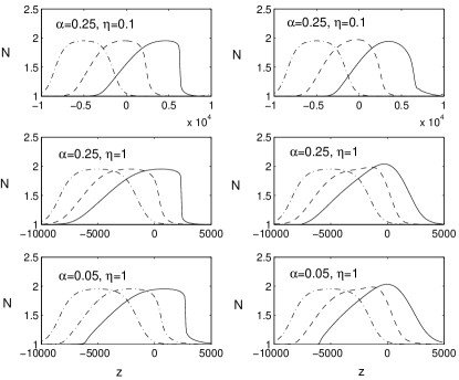
Figure 2: The profile of the ion density $N$ obtained from numerical solutions of the fluid equations (left panels) and the Vlasov equation (right panels). In the upper panels, the profiles are shown at $t=0$ (dash-dotted lines), $t=1700$ (dashed lines) and $t=3400$ (solid lines), while in the middle and lower panels the profiles are shown at $t=0$, $t=500$ and $t=1000$. Parameters are $\eta=0.1$ and $\alpha=0.25$ (upper panels), $\eta=1$ and $\alpha=0.25$ (middle panels) and $\eta=1$ and $\alpha=0.05$ (lower panels).

In Fig. 2, we present a comparison between the density profiles obtained from the fluid and Vlasov simulations, at different times. In the upper panel, the ion-electron temperature ratio $\eta=0.1$, and the electron-ion density ratio $\alpha=0.25$. We see that both the fluid (left) and Vlasov (right) solutions exhibit shocks, where the shock front is distinct in the fluid solution and more diffuse in the Vlasov solution. The corresponding ion distribution function is displayed in Fig. 3.

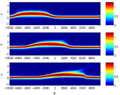
Figure 3: The ion distribution function at $t=0$ (upper panel), $t=1700$ (middle panel) and $t=3400$ (lower panel) as a function of $x$ and $v$. Parameters are $\eta=0.1$ and $\alpha=0.25$.

We observe that the formation of the shock at $t=3400$ is located at $z\approx 7000$. It is associated with a “kink” in the distribution function. A population of ions have also been accelerated by the shock. The middle panels of Fig 2 are for $\eta=0.1$ and $\alpha=0.25$. Here, the fluid solution exhibits clear shocks, while the Vlasov simulation shows only a phase of self-steepening at $t=500$, followed by an expansion of the diffuse shockfont at $t=1000$.

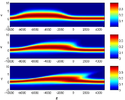
Figure 4: The ion distribution function at $t=0$ (upper panel), $t=500$ (middle panel) and $t=1000$ (lower panel) as a function of $x$ and $v$. Parameters are $\eta=1$ and $\alpha=0.25$.

The ion distribution function in Fig. 4 shows that the shockfront is strongly Landau damped for this case. Finally, the bottom panels of Fig. 2 show results for $\alpha=0.05$ and $\eta=1$. In this case, the fluid solution again shows a shock in the front end of the pulse, but also the rear end of the shock steepens, which can be seen at $z\approx-6000$ for $t=1000$. The steepening of the pulse for low-amplitude density perturbations in the rear of the pules can be explained by that the wave speed decreases for small-amplitude density perturbations ($N<1.1$), as seen in Fig. 1, while it increases again for large-amplitude density perturbations. The Vlasov solution again shows a diffusive shock in the front, while it reproduces the steepening of the density in the rear of the pulse.

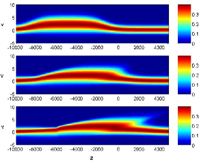
Figure 5: The ion distribution function at $t=0$ (upper panel), $t=500$ (middle panel) and $t=1000$ (lower panel) as a function of $x$ and $v$. Parameters are $\eta=1$ and $\alpha=0.05$.

In the middle panel of Fig. 5, the ion distribution function shows the self-steepening phase of the shockfront, and the lower panel shows the diffusion of the shock by shock-accelerated ions. In the rear end of the pulse, the distribution function forms a “kink,” clearly seen at $z\approx-6000$ in the bottom panel.

We have also performed simulations with smaller amplitudes of the pulses (not shown here) and they exhibit essentially the same behavior as in the large-amplitude case. It is interesting to note that it is the strongly heated and shock-accelerated ions in the pulse that leads to Landau damping by overtaking the pulse. The heating of the ions is due to adiabatic compression, leading to a higher thermal speed of the ions inside the pulse than in the equilibrium plasma. Another effect is that the fluid (mean) velocity of the ions further accelerates the ions. For Landau damping to be unimportant, we thus have the condition that the wave speed must be much larger than the sum of the ion thermal and fluid velocities. Inserting Eqs. (15) and (16) into the inequality $\lambda_{+}\gg V_{T}+u$, where the scaled ion thermal speed $V_{T}=(\eta T)^{1/2}\approx\eta^{1/2}N$, we obtain the condition $N^{1/2}[1/(N+\alpha-1)+3\eta N]^{1/2}\gg(\eta N^{2})^{1/2}$, or $(1/[(N+\alpha-1)N\eta]+3)^{1/2}\gg 1$. This condition is fulfilled if $\eta\ll 1$ (leading to the sharp shock seen in Fig. 3 and the upper right panel of Fig 2) or/and if the electrons are evacuated due to the dust so that $\alpha\ll 1$, and at the same time $N\approx 1$. The latter corresponds to the case where the sign of the coefficient in front of the low-amplitude nonlinear term becomes negative, so that there will be a shock in the rear end of the pulse while the front of the shock expands, in agreement with the observations in Fig. 5 and lower right panel of Fig 2. The expansion of the shockfront at high dust densities has also been observed in the experiment r3 .

To summarize, we have presented the dynamics of fully nonlinear, nondispersive dust ion acoustic waves in an unmagnetized dusty plasma. By using the Boltzmann electron distribution as well as the hydrodynamic equations for the warm ion fluid and quasi-neutrality condition, we have represented the governing equations in the form of a master equation whose characteristics have been found analytically. The fluid equations has been solved to obtain the density and velocity profiles of the DIA shock waves, which exhibit the steepening of the waveforms both in the front and rear depending upon the values of $\alpha$. We have also compared our theoretical results with those obtained from computer simulations of the time dependent Vlasov equation. The Vlasov solution shows a diffuse shock in the front end of the pulse, due to strong Landau damping, while a sharp shock develops in the rear end of the pulse, similar to the results from the simulation of Eqs. (5) and (6).

- (1) P. K. Shukla and V. P. Silin, Physica Scripta 45, 508 (1992).
- (2) A. Barkan, N. D’Angelo, and R. Merlino, Planet. Space Sci. 44, 239 (1996); R. L. Merlino, A. Barkan, C. Thompson, and N. D’Angelo, Phys. Plasmas 5, 1607 (1998).
- (3) Y. Nakamura, H. Bailung, and P. K. Shukla, Phys. Rev. Lett. 83, 1602 (1999).
- (4) Q.-Z. Luo and R. L. Merlino, Phys. Plasmas 6, 3455 (1999).
- (5) Q.-Z. Luo, N. D’Angelo, and R. L. Merlino, Phys. Plasmas 7, 2370 (2000).
- (6) Y. Nakamura, Phys. Plasmas 9, 440 (2002).
- (7) P. K. Shukla, Phys. Plasmas 7, 1044 (2000).
- (8) A. A. Mamun and P. K. Shukla, Phys. Plasmas 9, 1468 (2002).
- (9) P. K. Shukla and A. A. Mamun, Introduction to Dusty Plasma Physics (Institute of Physics, Bristol, UK, 2002).
- (10) S. I. Popel, A. P. Golub, and T. V. Losseva, JETP Lett. 74, 362 (2001).
- (11) B. Eliasson and P. K. Shukla, Formation of large amplitude dust ion-acoustic shocks in dusty plasmas, Phys. Plasmas (submitted 2004).
- (12) D. Montgomery, Phys. Rev. Lett. 19, 1465 (1967).
- (13) R. Bharuthram and P. K. Shukla, Planet. Space Sci. 40, 973 (1992).