Karhunen-Loeve analysis of complex spatio-temporal dynamics of thin-films optical system

Abstract

Application of Karhunen-Loeve decomposition (KLD, or singular value decomposition) is presented for analysis of the spatio-temporal dynamics of wide-aperture vertical cavity surface emitting laser (VCSEL), considered as a thin-layer system. KLD technique enables to extract a set of dominant components from complex dynamics of system under study and separate them from noise and inessential underlying dynamical behavior. Properties of KLD spectrum and structure of its main components are studied for different regimes of VCSEL. Along with the analysis of VCSEL, a brief survey of KLD method and its usage for theoretical and experimental description of nonlinear dynamical systems is presented.

Key words: thin films, spatio-temporal dynamics, VCSEL, singular value decomposition, Karhunen-Loeve decomposition
PACS numbers: 42.55.Px; 42.60.Jf
UDC: 621.373.826.038+539.2

1 Introduction

Investigation of interaction of thin-film systems with laser radiation becomes quite topical during the last decade. This is mainly stimulated by advances of semiconductor technology, which enable to obtain multi-layer semiconductor structures with thickness close to or even less than wavelength of visible radiation. In particular, wide-aperture vertical cavity surface emitting lasers (VCSELs) are wide-spread optical systems of communication and information processing. Complex spatio-temporal regimes of VSCEL operation, in principle, opens new possibilities for information processing (for example, “chaotic” encoding for secure applications). On the other hand, it is far from full understanding, what mechanisms form spatial and temporal structure of radiation in VCSELs.

In the paper, we investigate the spatiotemporal dynamics of VCSEL using the system of differential equations describing the dynamics of broad area VCSEL [1]. The equations are derived using spin flip model [2, 3] and take into account polarization of light and complex cavity of VCSEL, including Bragg reflectors. The propagation of radiation through the VCSEL cavity is calculated in an approximation of thin nonlinear layer, which allows to dismiss the diffraction of light in the active medium. Calculations of the current intensity $J$ near threshold and for some values far from threshold are performed for the case of zero phase anisotropy, low amplitude anisotropy and homogeneous spatial profiles of refraction index and injection current.

Obtained sets of spatiotemporal data are analyzed using Karhunen-Loéve decomposition (KLD, also known by several other names [4]). Such technique is introduced in the beginning of 20th century for description of random functions. Then this method have found numerous applications in such areas as pattern recognition, turbulence, meteorology, coherence theory etc. Optimal properties of KLD enables to extract only a few main components from the whole complex dynamics of system under study.

The rest of article is organized as follows: in the next section we outline the method of or Karhunen-Loéve decomposition and its main characteristics. In the third section we provide the mathematical model of VCSEL is presented. In the following section we analyze of complex dynamics of VCSEL by KLD method. In particular, change of the decomposition spectrum for the values of the current density $J$ near lasing threshold and for some values above threshold is discussed. The last section contains a conclusion and outline of future tasks.

2 Karhunen-Loéve decomposition

In its simplest form, suitable for our purposes, the KLD method is formulated as follows: given some (in general, complex) field of two variables $u(\mathbf{r},t)$ with $\mathbf{r}=(x,y)$, one tries to find its decomposition onto purely temporal and spatial modes:

$$u(r,t)=\sum_{i=1}^{\infty}\lambda_{i}\,a_{i}(t)\,\phi_{i}(\mathbf{r}).$$ (1)

with two orthonormality conditions

$$\int_{S}d\mathbf{r}\;\phi_{i}(\mathbf{r})\,\phi^{\ast}_{j}(\mathbf{r})=\delta_{ij}\qquad\int_{T}dt\;a_{i}(t)\,a^{\ast}_{j}(t)=\delta_{ij}$$ (2)

where $T$ is a time interval and $S$ is an area on which we want to analyze field. This field is considered as known, e.g. from experiment, or from some kind of model - either analytical or numerical.

The physical sense of representation (1) is extraction of spatial distributions which oscillate in time as a whole. The values $|\lambda_{i}|^{2}$ give the part of ‘energy’ carried by $i$-th mode in average. Physical origin of $u(\mathbf{r},t)$ is of little importance — it could be electrical field or intensity of some kind of radiation, velocity profile of flow or even simply set of pictures $u(\mathbf{r})$ numbered by second variable $t$ [5, 6]. In our case, $u(\mathbf{r})$ is the slowly varied complex envelope of the optical field. One of the main parameters of presentation (1) is the number of terms $N_{\epsilon}$, such that their sum contains not less that some prescribed part of the whole energy of $u(\mathbf{r},t)$

$$\sum_{i=1}^{N_{\epsilon}}|\lambda_{i}|^{2}\geqslant(1-\epsilon)\sum_{i=1}^{\infty}|\lambda_{i}|^{2}.$$ (3)

The other components with $i>N_{\epsilon}$ bears noise or unimportant dynamics and so could be excluded from consideration (on given interval of time and spatial domain).

As it could be shown, the decomposition functions could be found from two eigenproblems for integral equations

$$|\lambda_{i}|^{2}\,\psi_{i}(\mathbf{r})=\int_{S}d\mathbf{r}^{\prime}\;\phi_{i}(\mathbf{r}^{\prime})\,K_{S}(\mathbf{r},\mathbf{r}^{\prime})$$ (4)

and

$$|\lambda_{i}|^{2}\,a_{i}(t)=\int_{T}dt^{\prime}\;a_{i}(t^{\prime})\,K_{t}(t,t^{\prime})$$ (5)

where kernels are correlation function

$$K_{S}(\mathbf{r},\mathbf{r}^{\prime})=\int_{T}dt\;u(\mathbf{r},t)\,u(\mathbf{r}^{\prime},t)$$ (6)

and some kind of temporal correlation function, averaged over space

$$K_{S}(\mathbf{r},\mathbf{r}^{\prime})=\int_{T}dt\;u(\mathbf{r},t)\,u(\mathbf{r}^{\prime},t).$$ (7)

Equation (5) with kernel (7) is usually referred to as “method of snapshots” of “method of strobes” [4].

On the other hand, decomposition of type (1), (2) corresponds to singular-value decomposition [7] of “matrix” $u(\mathbf{r},t)$. As far as experimental (or numerical calculation) data is always is a kind of matrix of numbers. Appropriate discrete decomposition may be effectively calculated using standard svd routine available in umber of mathematical packages.

It should be noted, that whole decomposition could be found from just one eigenproblem, while the dual basis, temporal or spatial, is found from projection

$$\lambda_{i}\,a_{i}(t)=\int_{S}d\mathbf{r}\;\phi^{\ast}_{i}(\mathbf{r})\,u(\mathbf{r},t),$$

$$\lambda_{i}\,\psi_{i}(\mathbf{r})=\int_{T}dt\;a^{\ast}_{i}(t)\,u(\mathbf{r},t).$$

Use of eigenfunctions related to the investigated field cause main positive sides of Karhunen-Loéve expansion: among all sums of type (1) with finite number of terms, the representation in terms of eigenfunctions ensures minimal least square error and the maximal capture of ”energy.” The KLD method proves its power on number of problems in different areas of physics and other sciences. On the other hand, its main drawback again related with use of eigenfunctions: analytical solution of equations (4), (5) is known only for very few special cases, the numerical solution often require too much resources and is incapable to provide all the information about system dynamics, especially near critical points. To this point, it is important to look for methods of analysis, which provide information about spectrum of eigenvalues $|\lambda|^{2}$ without calculation of decomposition itself [8].

However, calculation of Karhunen-Loéve decomposition provides valuable information about the details of complex process. Solution of eigenvalue problem is usually much more easy task than to study other, “standard” parameters of chaotic systems, such as Lyapunov exponents or fractal dimensions. In most cases singular-value analysis enables to select just the few most important components from whole spatio-temporal dynamics and to study their behaviour.

3 Short description of the VCSEL model

Response of the active medium to the radiation in VCSEL is in a semiclassical approximation is described by the spin-flip model [2, 3, 1], taking into account vector character of field:

$$\left\{\begin{aligned} \frac{d\mathbf{P}}{dt}&=-\left(\frac{1}{T_{2}}+i\delta\right)P-\frac{|d|^{2}}{3\overline{h}}iA\mathbf{E},\\ \frac{N}{dt}&=-\frac{N-J}{T_{1}}-\frac{i}{2\overline{h}}\left(\mathbf{E^{*}}\mathbf{P}-\mathbf{E}\mathbf{P^{*}}\right),\\ \frac{n}{dt}&=-\gamma_{s}n+\frac{1}{2\overline{h}}\left(\mathbf{E^{*}}\mathbf{P^{\prime}}-\mathbf{E}\mathbf{P^{\prime*}}\right).\end{aligned}\right.$$ (8)

where $\mathbf{P}$ is the polarization of the two level centers, $\mathbf{P^{\prime}}$ is the vector with components $(P_{y},-P_{x})$; $N$ is the total population difference between the conduction and the valence bands and $N_{0}$ is its transparency value; $n$ is the difference between the population differences for the two allowed transitions between magnetic sublevels, $\delta=\omega_{g}-\omega_{c}$ is the detuning between the bandgap frequency $\omega_{g}$ and the cavity resonance $\omega_{c}$; $\gamma_{s}$ is the decay rate between the magnetic sublevels; $T_{1}$ and $T_{2}$ are the relaxation times for the total population difference and the polarization correspondingly; $|d|$ is the absolute value of the dipole momentum of the transition (we suppose it is the same for both transitions); $J$ is the pump parameter, and

$$A=\left(\begin{array}[]{cc}N-N_{0}&in\\ -in&N-N_{0}\end{array}\right).$$ (9)

We will use equations (8) with adiabatically eliminated polarization. The procedure of such adiabatic elimination is described in details in [1] and allows to take into account the asymmetry of the gain line using so called linewidth enhancement factor $\alpha$. In addition, this procedure allows to avoid the short-frequency instabilities intrinsic to the straightforward adiabatic elimination procedure for the spatially extended lasers. In this approximation the polarization of the active medium is defined as follows:

$$P=-\frac{|d|^{2}T_{2}}{3\overline{h}}(i-\alpha)D\hat{\pounds}\mathbf{E},$$ (10)

here $D=N-N_{0}$, the operator $\hat{\pounds}\sim\pounds(\vec{k}_{\perp})=1/[1+T_{2}^{2}(\delta-\Omega(\vec{k}_{\perp}))^{2}]$, where $\Omega(\vec{k}_{\perp})$ is a cavity resonance frequency for the tilted wave with definite $\vec{k_{\perp}}$, and the tilde means an equivalence in the sense of transverse Fourier transform.

The propagation of radiation through the VCSEL cavity is calculated in an approximation of thin film active medium, which allows to neglect the diffraction in an active layer [1]. It gives us the following relation:

$$\mathbf{E_{i}}=\hat{F}\>\mathbf{E_{t}}.$$ (11)

where $\mathbf{E_{i}}$ is the field incident into the active medium, $\mathbf{E_{t}}$ is the field outgoing from the active medium. Operator $\hat{F}=\rho\,\exp({2ikL+i(\Delta_{\perp}/k)L})\,\Gamma\,\hat{R}$, where $\rho$ describes absorption in the linear medium between the active layer and reflector, $L$ is the thickness of the spacer layer, $\Delta_{\perp}$ is the Laplasian in the transverse plane,

$$\Gamma=\left(\begin{array}[]{cc}e^{\gamma_{a}+i\gamma_{p}}&0\\ 0&e^{-(\gamma_{a}+i\gamma_{p})}\end{array}\right),$$ (12)

is an polarization anisotropy matrix, with $\gamma_{a}$, $\gamma_{p}$ being the amplitude and phase anisotropy parameters correspondingly. Operator $\hat{R}$ describes the reflection of plane waves from the Brag reflectors [1].

For numerical simulations we used the following parameters: $\gamma_{s}=100$, $\gamma_{a}=0.1$, $\gamma_{p}=0.0$, $\delta=0.006$, $\alpha=3.0$. For chosen parameters the lasing threshold is $J_{0}=0.730$ which is needed for the following discussion (see [1] for the detailed description of threshold conditions).

4 Analysis of VCSEL dynamics

We consider first the simplest homogeneous case with periodic boundary conditions and with small amplitude anisotropy. The resulting spatiotemporal regime near threshold ($J=0.740$) is regular and consists of stripes that weakly oscillate near certain equilibrium state (the directions of oscillations is shown in Fig.1b by arrows). The contrast of stripes also changes during the evolution. The KL-spectra of eigenvalues $\lambda_{j}$ of the spatiotemporal regime for this case is presented in Fig.1a. It is evident, that only two modes are the most significant, while all the others could be safely treated as zeros.

The spatial KL-modes appear to be stripes (Fig.2). Their maxima don’t coincide and thus a spatial phase shift leads to orthogonality and to spatiotemporal dynamics. Hence, the averaging over a large period of time leads to stripes with smaller contrast. Time dependencies of the KL-modes (see Fig. 3) also characterized by regular (oscillating) dynamics, except only some transient stage.

However, a slight enlarge of the injection current (up to $J=0.800$) leads to chaotic time dependency the field. Nevertheless, in this case the KL-spectra has the same form as one near threshold Fig. 1a, and, moreover, the spatial KL-modes are the same as in Fig. 2 too. However, their temporal behavior is sufficiently different (see Fig.4).

Therefore, the chaotization of the regular dynamics appears due to mechanism, which is not connected with excitation of the long-wavelength inhomogenities, either Eckhaus or zig-zag type (i.e. in $x$ or $y$ directions).

Further increase of the injection current ($J=1.000$) leads to more disordered dynamics. More than two active modes are present in in KL-spectrum (Fig. 5). The spatial structure is also changing in this case, and modulation in $x$ direction now is accompanied by modulation in $y$ direction (see Fig. 6).

5 Conclusion

In summary, our calculations have shown, that during transition of VCSEL’s from the regular behavior to spatio-temporal chaos, it still can be described by superposition of just a few modes with relatively simple structure (for moderate values of the injection current). Increase of order parameter (injection current $J$) leads to activation of some new modes, with new features of transversal and temporal dependence.

Hence, the observed chaos is not truly “spatio-temporal”. Complex dynamics in time domain (both for the electomagnetic field itself and for KL-modes) is accompanied by just very simple spatial structure of modes. Moreover, the whole dynamics is described by only a few components. This fact, together with importance of VCSELs in modern optical communication, enables to suppose, that chaotic regimes could be effectively controlled by adjusting parameters of a system.

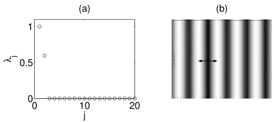
Figure 1: (a) - The KL spectra for J=0.740. (b) - The zoomed snapshoot of the dynamics. The arrows shows the direction of oscillations(the amplitude of oscillations is smaller then the length of arrows).

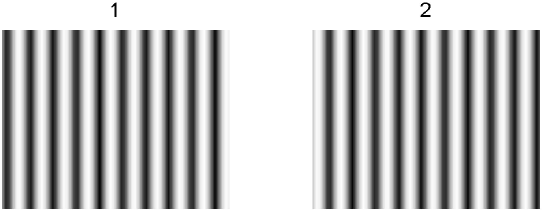
Figure 2: The first 2 spatial KL-modes for $J=0.740$.

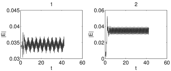
Figure 3: The temporal evolution of KL-modes shown in Fig. 2.

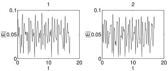
Figure 4: The first 2 temporal KL-modes for J=0.800.

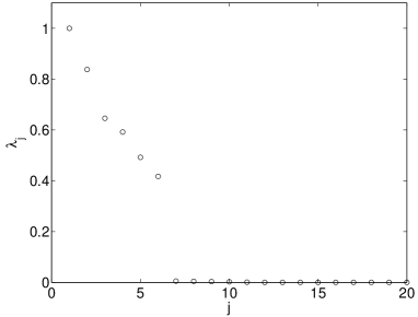
Figure 5: The KL spectra for J=1.000.

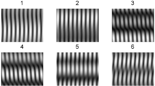
Figure 6: The first 6 spatial KL-modes for J=1.000.

References

- [1] N. A. Loiko and I.V. Babushkin, J.Opt. B: Quantum semiclass. Opt. vol. 3, p. S234 (2001).
- [2] M. San Miguel, Q. Feng, and J. V. Moloney, Phys. Rev. A, vol. 52, p. 1728 (1995).
- [3] J. Martin-Regalado, F. Prati, M. San Miguel, and N. B. Abraham, IEEE journal of quantum electronics, vol. 33, p. 765 (1997).
- [4] P. Holmes, J. L. Lumley, and G. Berkooz, ”Turbulence, coherent structures, dynamical systems and symmetry”, Cambridge university press, 1998.
- [5] R. Everson, L. Sirovich, J. Opt. Soc. Am. A., vol. 12, p. 1657 (1999).
- [6] O. M. Soloveyko, Y. S. Musatenko, V. N. Kurashov, V. A. Dubikovskiy, Proc. SPIE., vol. 4041, p. 180 (2000).
- [7] G. W. Stewart, SIAM Rev., vol. 35, p. 551 (1993).
- [8] A. M. Lazaruk, N. V. Karelin, Proc. SPIE., vol. 3317, p. 12 (1997), see also arXiv.org preprint physics/9712011.