Programming matrix optics into Mathematica

Abstract

The various non-linear transformations incurred by the rays in an optical system can be modelled by matrix products up to any desired order of approximation. Mathematica software has been used to find the appropriate matrix coefficients for the straight path transformation and for the transformations induced by conical surfaces, both direction change and position offset. The same software package was programmed to model optical systems in seventh-order. A Petzval lens was used to exemplify the modelling power of the program.

Keywords

Aberration, matrix optics, computer optics.

1 Introduction

In previous papers [1, 2] it was shown that it is possible to determine coefficients for matrix modelling of optical systems up to any desired order, computing power being the only limiting factor. The second of those paper lists the calculated seventh-order coefficients for systems comprising only spherical surfaces.

The use of matrices for optical modelling of optical systems under paraxial approximation is well known, see for instance [3]. Other authors have shown the possibility of extending matrix modelling to higher orders [4, 5] and the author has used in his previous work a different set of coordinates which made feasible the implementation of matrix models in personal computers.

The first part of the paper describes the calculations necessary for the determination of matrix coefficients and the manner these were performed with Mathematica software [6]. The programming is general for surfaces that can be described analytically and for whatever approximation is desired. The possibilities of the modelling system are then exemplified with the study of a Petzval lens’ aberrations.

A set of Mathematica functions needed for the implementation of matrix models was defined and assembled in a package which is described in its most relevant aspects in the appendix.

2 Determination of expansion coefficients

2.1 Initialization

In this section we explain how Mathematica can be used to evaluate all the expansion coefficients needed for further implementation of matrix models. The method is explained with great generality and can be used up to any degree of approximation and with all surfaces that can be defined analytically.

First of all we must load two packages that will be used further along:

 Needs["Calculus‘VectorAnalysis‘"]
 Needs["Optics‘expansion‘"]

The first package is distributed standard with Mathematica and is useful for performing vector operations. The second one is a proprietary package which performs series expansion in different way. The standard series expansion for multi-variable functions sets the limit for each variable’s exponent independently but not for the order of the monomials. The expansion package sets a limit for the monomials’ order, so that each variable’s exponent is adjusted accordingly; for details see appendix B.

2.2 Surface definition

The method is applicable to any surface which can be defined by an equation of the type $\mathrm{f}(x,y,z)=0$. For instance, a conic of revolution could be defined as:

 surface[x_, y_, z_] = Sqrt[x^2 + y^2 + z^2] + e*z - r;

We are going to need the normal to the surface at any point; this can be found applying gradient to the surface expression:

 n = Grad[surface[Xx, Yy, Zz], Cartesian[Xx,Yy,Zz]];

2.3 Snell’s law

Snell’s law is usually written as scalar relationship between sines of the angles the rays form with the normal on both sides of the surface, but it can also be expressed as a vector relationship using cross products [2]. Let us define to unit vectors representing the ray directions on the two sides of the surface:

 v = {s, t, Sqrt[1 - s^2 - t^2]};
 v1 = {s1, t1, Sqrt[1-s1^2-t1^2]};

v and v1 represent the unit vectors, s, t, s1 and t1 are direction cosines.

Snell’s law requires that the cross product of the ray direction with the surface normal, multiplied by the refractive index be equal on both sides:

$$u\,{\bf v}\otimes{\bf n}={\bf v1}\otimes{\bf n}~{},$$ (1)

where $u$ represents the refractive index ratio of the two media. We ask Mathematica to find the solutions of Eq. (1) for the surface in question:

 Snell = Solve[{u*CrossProduct[v, n] ==
       CrossProduct[v1, n],surface[Xx,Yy,Zz]==0}, {s1, t1,Zz}];

Eq. (1) has four solutions, corresponding to positive and negative angles, in the forward and the reverse directions. The solutions found by Mathematica must be scanned in order to find the appropriate one. We can write the exact solution with two commands:

 sd = Simplify[s1 /. Snell[[3]]]
 td = Simplify[t1 /. Snell[[3]]]

which will output very long expressions very impractical for use.

2.3.1 Series expansion

The solutions of Eq. (1) must be expanded in series to the desired order of approximation for which we use a function from the expansion package. Dealing with axis-symmetric systems it is useful to resort to complex coordinates; the two solutions are thus combined into one single complex solution, then expanded to the fifth order and simplified:

 sexpand = Expansion[sd + I*td, s, t, Xx, Yy, 5];
 sexpand = Simplify[PowerExpand[sexpand]];

The result of the Expansion function is a list of coefficients, most of them zero. The expansion package provides a function VectorBase which outputs a list of all the monomials that can be built with the given list of variables up to the desired order. This can be left-multiplied by the coefficient list in order to get a polynomial:

 sexpand = sexpand . VectorBase[s, t, x, y, 5];

2.3.2 Complex coordinates

Although combined into one single complex coordinate in sexpand, the output ray direction cosines are still expressed in terms of real input ray position and direction coordinates; this must be corrected by an appropriate coordinate change, followed by suitable manipulation and simplification:

 Apply[Plus,Simplify[MonomialList[ComplexExpand[sexpand /.
   {x -> (X + Conjugate[X])/2,
    y -> (X - Conjugate[X])/(2*I),
    s -> (S + Conjugate[S])/2,
    t -> (S - Conjugate[S])/(2*I)}, {X,S},
    TargetFunctions->Conjugate],
    {X, Conjugate[X], S, Conjugate[S]},
    CoefficientDomain->RationalFunctions]]]

Mathematica will output an expression for the above command, which is reproduced bellow in a slightly different form:

$$S\,u-{\frac{\left(1+u\right)\,X}{r}}+{\frac{S\,u\,\left(1+u\right)\,X\,\mathrm{Conjugate}(S)}{2\,r}}-{\frac{u\,\left(1+u\right)\,{X^{2}}\,\mathrm{Conjugate}(S)}{2\,{r^{2}}}}$$

$$+{\frac{{S^{2}}\,\left(u+{u^{4}}\right)\,X\,{{\mathrm{Conjugate}(S)}^{2}}}{8\,r}}-{\frac{S\,{u^{2}}\,\left(-1+{u^{2}}\right)\,{X^{2}}\,{{\mathrm{Conjugate}(S)}^{2}}}{4\,{r^{2}}}}$$

$$+{\frac{{u^{2}}\,\left(-1+{u^{2}}\right)\,{X^{3}}\,{{\mathrm{Conjugate}(S)}^{2}}}{8\,{r^{3}}}}-{\frac{S\,u\,\left(1+u\right)\,X\,\mathrm{Conjugate}(X)}{2\,{r^{2}}}}$$

$$+{\frac{\left(1+u\right)\,\left({e^{2}}+u\right)\,{X^{2}}\,\mathrm{Conjugate}(X)}{2\,{r^{3}}}}$$

$$-{\frac{{S^{2}}\,{u^{2}}\,\left(-1+{u^{2}}\right)\,X\,\mathrm{Conjugate}(S)\,\mathrm{Conjugate}(X)}{4\,{r^{2}}}}$$

$$-{\frac{S\,u\,\left(1+u\right)\,\left(1+{e^{2}}+2\,u-2\,{u^{2}}\right)\,{X^{2}}\,\mathrm{Conjugate}(S)\,\mathrm{Conjugate}(X)}{4\,{r^{3}}}}$$

$$+{\frac{u\,\left(1+u\right)\,\left(2\,{e^{2}}+u-{u^{2}}\right)\,{X^{3}}\,\mathrm{Conjugate}(S)\,\mathrm{Conjugate}(X)}{4\,{r^{4}}}}$$

$$+{\frac{{S^{2}}\,{u^{2}}\,\left(-1+{u^{2}}\right)\,X\,{{\mathrm{Conjugate}(X)}^{2}}}{8\,{r^{3}}}}$$

$$+{\frac{S\,u\,\left(1+u\right)\,\left(2\,{e^{2}}+u-{u^{2}}\right)\,{X^{2}}\,{{\mathrm{Conjugate}(X)}^{2}}}{4\,{r^{4}}}}$$

$$+{\frac{\left(1+u\right)\,\left(-3\,{e^{4}}+u-6\,{e^{2}}\,u-{u^{2}}+{u^{3}}\right)\,{X^{3}}\,{{\mathrm{Conjugate}(X)}^{2}}}{8\,{r^{5}}}}$$

All the coefficients resulting from similar operations performed on a spherical surface up to the seventh order have already been listed by the author [2] and the reader is referred to that work for further elucidation.

2.4 Surface offset

We will now deal with the problem of the offset introduced by the surface on the position coordinates; the reader is again referred to the above mentioned work for full explanation of this matter.

Mathematica will respond quicker if we perform shift the coordinate origin, along the axis, to the geometrical centre of the surface; this is the purpose of the three following commands:

 eq = Solve[surface[x, y, z] == 0, z],
 z1 = z /. eq[[2]];
 z1 = z1 - r/(-1 + e);

The ray coordinates on the point of incidence will have to obey the two equations:

$$x1 = x+{\frac{sz1}{\sqrt{1-s^{2}-t^{2}}}}~{};$$

$$y1 = y+{\frac{tz1}{\sqrt{1-s^{2}-t^{2}}}}~{}.$$ (2)

The following commands will perform the necessary calculations:

 eqx = x1 == x + s*z1/Sqrt[1 - s^2 - t^2];
 eqy = y1 == y + t*z1/Sqrt[1 - s^2 - t^2];
 offset = Solve[{eqx, eqy}, {x, y}];

The ray will usually intersect a surface in two points but complex surfaces can be intersected in several points; the relevant solution is the one that is closest to the surface vertex plane, which will have to be selected from the multiple solutions found by Mathematica:

 xd = Simplify[x /. offset[[2]]];
 yd = Simplify[y /. offset[[2]]];

2.4.1 Series expansion

The commands that follow reproduce a procedure similar to what was explained in paragraphs 2.3.1 and 2.3.2:

 xexpand =
  Simplify[PowerExpand[Expansion[xd + I*yd, s,
     t, x1, y1, 5]],TimeConstraint->Infinity];
 xexpand = xexpand . VectorBase[s, t, x, y, 5];
 Simplify[MonomialList[ComplexExpand[xexpand /.
   {x -> (X + Conjugate[X])/2,
    y -> (X - Conjugate[X])/(2*I),
    s -> (S + Conjugate[S])/2,
    t -> (S - Conjugate[S])/(2*I)}, {X,S},
    TargetFunctions->Conjugate],
    {X, Conjugate[X], S, Conjugate[S]},
    CoefficientDomain->RationalFunctions]]

The result is the following coefficient list:

$$\{ {\frac{\left(-1+{e^{2}}\right)\,S\,{X^{2}}\,{{\mathrm{Conjugate}(X)}^{2}}}{8\,{r^{3}}}},$$

$${\frac{S\,{X^{2}}\,\mathrm{Conjugate}(S)\,\mathrm{Conjugate}(X)}{4\,{r^{2}}}},$$

$${\frac{{S^{2}}\,X\,{{\mathrm{Conjugate}(X)}^{2}}}{4\,{r^{2}}}},$$

$${\frac{-\left({S^{2}}\,X\,\mathrm{Conjugate}(S)\,\mathrm{Conjugate}(X)\right)}{4\,r}},$$

$${\frac{-\left(S\,X\,\mathrm{Conjugate}(X)\right)}{2\,r}},X\,\}$$

The complete set of coefficients for the seventh-order and spherical surfaces can be found on the paper mentioned before. The same reference lists the coefficients for the reverse offset, which are determined in an entirely similar manner.

2.5 Straight path

The use of direction cosines to define the ray orientation renders a straight path into a non-linear transformation, whose expansion must also be taken care of. The procedure is similar to what was used above and there are no mathematical complexities involved; we will just list the commands and the final result:

 xexpand =
  Simplify[PowerExpand[Expansion[x +
      s*e/Sqrt[1 - s^2 - t^2] +
      I*(y + t*e/Sqrt[1 - s^2 - t^2]), s, t, x,
     y, 5]]];
 xexpand = xexpand . VectorBase[s, t, x, y, 5];
 Apart[xexpand /.
   {x -> (X + Conjugate[X])/2,
    y -> (X - Conjugate[X])/(2*I),
    s -> (S + Conjugate[S])/2,
    t -> (S - Conjugate[S])/(2*I)}, r]

The final output is:

$${\frac{1}{8}\left({8\,e\,S+8\,X+4\,e\,{S^{2}}\,\mathrm{Conjugate}(S)+3\,e\,{S^{3}}\,{{\mathrm{Conjugate}(S)}^{2}}}\right)}$$

3 Simulation of a Petzval lens

Figure 1: Diagram of a Petzval lens.

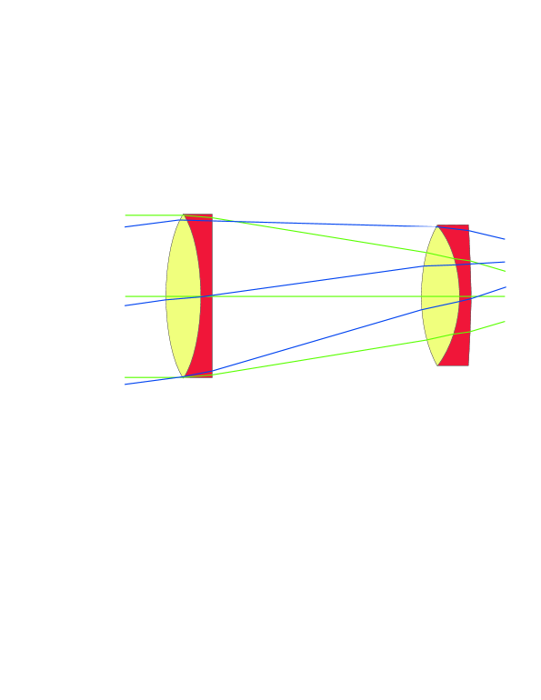
In this section we will use Mathematica to model a complex lens using matrix optics. The chosen lens is a Petzval design distributed with Oslo LT [7], which reproduces an example from Walker [8]; this lens is illustrated in Fig. 1 and is built with four elements made of glasses BK7 and SF4.

3.1 Initialization

The model uses a proprietary package named Sphericl which defines all the functions needed for implementation of matrix models of spherical systems, along with some other useful functions. The package is described in appendix A.

 Needs["Optics‘Sphericl‘"]

The two glasses used for the individual elements are defined by lists of their refractive indices at three wavelengths, namely 587.56 nm, 486.130 nm and 656.270 nm:

 bk7 = {1.5168, 1.522376, 1.514322};
 f4 = {1.616592, 1.62848, 1.611645};

3.2 Lens definition

The two functions Lens[] and Distance[] provide the matrices corresponding to the ray transformations induced by a single element in air and a straight path; they are multiplied successively, in reverse order relative to the transformations, in order to model the lens:

 Table[lens[i] =
    Lens[f4[[i]],-18.44,-40.23,3] . Distance[35] .
    Lens[bk7[[i]],41.42,103.08,8] . Distance[25] .
    Lens[bk7[[i]],-72.05,-92.6,7] . Distance[4] .
    Lens[bk7[[i]],53.12,-799.9,10] . Distance[60],{i,1,3}];

The last factor, Distance[60], corresponds to the distance from the aperture stop to the first surface. The Table[] function is used to generate models for all three wavelengths.

3.3 Image coordinates

The optimization performed by Oslo determined an image plane position at 3.787202 mm from the last surface, so there is one last product to make in order to find the overall system matrices for the three wavelengths:

 Table[image[i] = Distance[3.787202].lens[i],{i,1,3}];

The system matrices must be right-multiplied by the vector base in order to generate the coordinates and the higher order monomials for the image plane. The function Terms[] is responsible for generating a complex vector base from the given coordinates:

 Table[imagex[i]=(image[i].Terms[{x,s}])[[1]],{i,1,3}];

List imagex[i] is a 3 element vector, whose elements are the complex position coordinates for each of the three wavelengths. We can isolate the tangential and sagittal components by making the input coordinate real or imaginary and simultaneously taking the real or imaginary parts, respectively:

 Table[timage[i]=ComplexExpand[Re[imagex[i]]],{i,1,3}];
 Table[simage[i]=ComplexExpand[Im[imagex[i]/. x->I x]],{i,1,3}];

3.4 Ray analysis

         

Figure 2: Ray intercept curves for three wavelengths: green line – 587.56 nm, blue line – 486.130 nm, red line – 656.270 nm. Left figure is for on-axis incidence, right figure for $5^{\mathtt{o}}$ field angle.

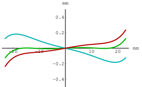
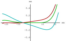
Finally we perform some ray analysis by plotting ray intercept curves for two different values of the field given by the variable s; the results are shown in Fig. 2:

 Table[timage0 = timage[1] /. x -> 0;
  Plot[{timage[1] - timage0, timage[2] - timage0,
      timage[3] - timage0}, {x, -23, 23},
    PlotRange -> {Automatic, {-0.5, 0.5}},
    PlotStyle -> {{AbsoluteThickness[2],
          RGBColor[0, 0.7, 0]}, {AbsoluteThickness[2],
          RGBColor[0, 0.7, 0.7]}, {AbsoluteThickness[2],
          RGBColor[0.7, 0, 0]}}, AxesStyle -> AbsoluteThickness[1],
    AxesLabel -> {"mm", "mm"}], {s, 0, 0.09, 0.087155}]

4 Conclusion

All the calculations needed for matrix modelling optical systems were successively programmed with Mathematica without limitations for surface shapes or degree of approximation. The program for the determination of series expansion coefficients was run in less than one hour for the seventh-order and spherical surfaces. Other surface shapes have already bean used and these include conicals and toroids.

After calculation, the coefficients have been incorporated in a Mathematica package which runs fast and avoids the need to re-calculate over and over. This package is fast and allows the simulation of very complex optical systems; one such example was demonstrated in the form of a Petzval lens.

Work is now going on to extract more possibilities from the software, namely for plotting wavefronts and ray-densities, and will be the object of other publications.

Appendix A The ”Sphericl” package

This package provides all the functions needed for the implementation of seventh-order matrix models of optical systems. Some auxiliary functions are also defined in order to facilitate other optical system calculations. This appendix describes in detail the fundamental functions and gives only short mentions of the others.

The package makes use of the axis symmetry to reduce matrix size to $40\times 40$, so all the coordinates are assumed to be complex. One ray, at any specific position is characterized by one complex position coordinate and on complex direction cosine coordinate.

Terms[]

The function builds the 40-element vector base with all the coordinate monomials that have non-zero coefficients in axis-symmetric systems:

 Terms[r_List] := Module[{x,s,ray},
 s = r[[2]] ; x = r[[1]]; ray = {x, s, x^2*Conjugate[x],
 x^2*Conjugate[s], s*x*Conjugate[x],
  s*x*Conjugate[s], s^2*Conjugate[x], s^2*Conjugate[s],
  x^3*Conjugate[x]^2, x^3*Conjugate[s]*Conjugate[x],
  x^3*Conjugate[s]^2, s*x^2*Conjugate[x]^2,
  s*x^2*Conjugate[s]*Conjugate[x], s*x^2*Conjugate[s]^2,
  s^2*x*Conjugate[x]^2, s^2*x*Conjugate[s]*Conjugate[x],
  s^2*x*Conjugate[s]^2, s^3*Conjugate[x]^2,
  s^3*Conjugate[s]*Conjugate[x], s^3*Conjugate[s]^2,
  x^4*Conjugate[x]^3, x^4*Conjugate[s]*Conjugate[x]^2,
  x^4*Conjugate[s]^2*Conjugate[x], x^4*Conjugate[s]^3,
  s*x^3*Conjugate[x]^3, s*x^3*Conjugate[s]*Conjugate[x]^2,
  s*x^3*Conjugate[s]^2*Conjugate[x], s*x^3*Conjugate[s]^3,
  s^2*x^2*Conjugate[x]^3,
  s^2*x^2*Conjugate[s]*Conjugate[x]^2,
  s^2*x^2*Conjugate[s]^2*Conjugate[x],
  s^2*x^2*Conjugate[s]^3, s^3*x*Conjugate[x]^3,
  s^3*x*Conjugate[s]*Conjugate[x]^2,
  s^3*x*Conjugate[s]^2*Conjugate[x], s^3*x*Conjugate[s]^3,
  s^4*Conjugate[x]^3, s^4*Conjugate[s]*Conjugate[x]^2,
  s^4*Conjugate[s]^2*Conjugate[x], s^4*Conjugate[s]^3};
 ray];

otherlines[]

All the transformation matrices have a common structure characterized by two lines of series expansion coefficients followed by thirty eight lines of elements derived from the former by algebraic operations. The otherlines[] function is an internal function which accepts as input any $40\times 40$ matrix and outputs another matrix with the same first two lines and lines 3 to 40 built according to the common rules.

It is impossible to list all the implementation lines for this function, for reasons of size; we will then resort to an explanation of the procedures for determining the coefficients for one of the 38 lines.

Suppose we want to find the coefficients for a line which corresponds to the monomial $X^{j}\mathrm{Conjugate}\left[X\right]^{k}S^{l}\mathrm{Conjugate}\left[S\right]^{m}$. We start be defining a square matrix t of dimension 40, with known elements on the first two rows:

 t = IdentityMatrix[40];
 t[[1]]=Table[a[i],{i,1,40}];
 t[[2]]=Table[b[i],{i,1,40}];

The matrix is right-multiplied by the vector base of coordinate monomials and the first two elements of the product are isolated:

 X1 = (t . Terms[{X, S}])[[1]];
 S1 = (t . Terms[{X, S}])[[2]];

The procedure then involves determining the product

 X1^j Conjugate[X1]^k S1^l Conjugate[S1]^m

and selecting just the terms up to the seventh order. The same procedure must be repeated for all the 38 lines.

These are lengthy calculations which must be performed only once. The function otherlines[] incorporates the results of those calculations and is fast to operate.

refraction[]

This is an internal function which receives as input the refractive indices of the two media and the curvature radius and outputs a transformation matrix whose second line contains the expansion coefficients for Snell’s law according to paragraph 2.3:

 refraction[n1_, n2_, r_] := Module[{matrix,u},
 matrix = IdentityMatrix[40];
 u=n1/n2;
 matrix[[2]] =
 {(u-1)/r,u,(u^2-u)/(2 r^3),(u^2-u)/(2 r^2),(u^2-u)/(2
 r^2),(u^2-u)/(2 r),0,0, (u^4-u)/(8 r^5),(u^4-u^2)/(4
 r^4),(u^4-u^2)/(8 r^3),(u^4-u^2)/(4 r^4),u(2u^3-3 u + 1)/(4 r^3),
 (u^4 - u^2)/(4 r^2),(u^4-u^2)/(8 r^3),(u^4-u^2)/(4 r^2),(u^4-u)/(8
 r),0,0,0, (u^6-u)/(16 r^7),u^2 (3u^4 - 2u^2 - 1)/(16 r^6),3
 u^4(u^2-1)/(16 r^5),(u^6-u^4)/(16 r^4), u^2(3 u^4-2 u^2-1)/(16
 r^6),u(9u^5-10u^3 + 1)/(16 r^5),u^2(9 u^4- 11 u^2 + 2)/(16 r^4), 3
 u^4(u^2-1)/(16 r^3),3 u^4(u^2-1)/(16 r^5),u^2(9 u^4-11 u^2+2)/(16
 r^4), u(9 u^5-10 u^3+1)/(16 r^3),u^2(3 u^4-2 u^2-1)/(16
 r^2),u^4(u^2-1)/(16 r^4),3 u^4(u^2-1)/(16 r^3), u^2(3 u^4-2
 u^2-1)/(16 r^2),u(u^5-1)/(16 r),0,0,0,0};
 otherlines[matrix]];

Screen[]

This is an external function which is used internally to determine the surface offset and externally to deal with spherical image surfaces. The structure is similar to the previous one but now its the first line which is defined:

 Screen[r_] := Module[{matrix},
 matrix = IdentityMatrix[40];
 matrix[[1]] = {1,0,0,0,1/(2r),0,0,0,0,0,0,
 1/(8 r^3),0,0,0,1/(4 r),0,0,0,0,0,0,0,0,1/(16
 r^5),0,0,0,0,1/(16 r^3),0,0,0,0,3/(16 r),0,0,0,0,0};
 otherlines[matrix]];

back[]

This is an internal function used to determine the reverse offset.

 back[r_] := Module[{matrix},
 matrix = IdentityMatrix[40];
 matrix[[1]] = {1,0,0,0,-1/(2r),0,0,0,0,0,0,
 -1/(8 r^3),1/(4 r^2),0,1/(4 r^2),-1/(4r),
 0,0,0,0,0,0,0,0,-1/(16 r^5),3/(16 r^4),
 -1/(8 r^3),0,3/(16r^4),-7/(16 r^3),1/(4 r^2),
 0,-1/(8 r^3),1/(4 r^2),-3/(16r),0,0,0,0,0};
 otherlines[matrix]];

Surface[]

This is an external function which receives as input the refractive indices of the two media and outputs the transformation matrix for a surface; it is built as the product of three matrices:

 Surface[n1_, n2_, r_] :=
 back[r] . refraction[n1, n2, r] . Screen[r];

Distance[]

This is an external function which receives as input the distance travelled along the axis and outputs the matrix for the straight path transformation:

 Distance[t_] := Module[{matrix},
 matrix = IdentityMatrix[40];
 matrix[[1]] = {1,t,0,0,0,0,0,t/2,0,0,0,0,0,
 0,0,0,0,0,0,3t/8,0,0,0,0,0,0,0,0,0,0,0,0,0,
 0,0,0,0,0,0,5 t/16};
 otherlines[matrix]];

Other functions

Auxiliary functions include Lens[], for the matrix of a single element lens in air, functions for gaussian constants, conjugates, etc.

Appendix B The ”expansion” package

BeginPackage["Optics‘expansion‘"]

Expansion::usage =
    "Expansion[e,{x,y,z,t},o] finds the coefficients of the series
    expansion of expression e in variables x,y,z,t up to the order o";


Begin["‘Private‘"];

Expansion[a_, {ax_, ay_, rx_, ry_}, o_] :=
    Module[{final, ser1, ser2, ser3, ser4}, final = 0;
      ser1 = Series[a, {ax, 0, o}];
      For[i = 0, i < o + 1, i++,
        ser2 = Series[Coefficient[ser1, ax, i], {ay, 0, o}];
        For[j = 0, j < o + 1 - i, j++,
          ser3 = Series[Coefficient[ser2, ay, j], {rx, 0, o}];
          For[k = 0, k < o + 1 - i - j, k++,
            ser4 = Series[Coefficient[ser3, rx, k], {ry, 0, o}];
            For[u = 0, u < o + 1 - i - j - k, u++,
              final=final+Coefficient[ser4,ry,u]*ax^i*ay^j*rx^k*ry^u;
              ]]]]; final]



End[]; EndPackage[];

References

- [1] J. B. Almeida, “The use of matrices for third order modeling of optical systems,” in International Optical Design Conference, K. P. Thompson and L. R. Gardner, eds., vol. 3482 of Proc. SPIE, pp. 917–925, 1998.
- [2] J. B. Almeida, “General method for the determination of matrix coefficients for high order optical system modeling,” J. Opt. Soc. Am. A 16, pp. 596–601, 1999.
- [3] A. Gerrard and J. M. Burch, Introduction to Matrix Methods in Optics, Dover Publications, New York, 1994.
- [4] M. Kondo and Y. Takeuchi, “Matrix method for nonlinear transformation and its application to an optical lens system,” J. Opt. Soc. Am. A 13, pp. 71–89, 1996.
- [5] V. Lakshminarayanan and S. Varadharajan, “Expressions for aberration coefficients using nonlinear transforms,” Optom. and Vision Sci. 74, pp. 676–686, 1997.
- [6] “Mathematica 3.0.” Wolfram Research, Inc., 1997.
- [7] “Oslo LT – version 5.” Sinclair Optics, Inc., 1995. Optics design software.
- [8] B. H. Walker, Optical Engineering Fundamentals, McGraw–Hill, 1995.