Callen’s Adiabatic Piston and the Limits of the Second Law of Thermodynamics

Abstract

The limits of the Second Law of Thermodynamics, which reigns undisputed in the macroscopic world, are investigated at the mesoscopic level, corresponding to spatial dimensions of a few microns. An extremely simple isolated system, modeled after Callen’s adiabatic piston, Callen60 can, under appropriate conditions, be described as a self-organizing Brownian motor and shown to exhibit a perpetuum mobile behavior.

I Introduction

As first clearly stated by Schroedinger “a living organism tends to approach the dangerous state of maximum entropy, which is death. It can only keep aloof from it, i.e., alive, by continually drawing from its environment negative entropy. What an organism fed upon is negative entropy”.Schroedinger45 Is it possible for an organism immersed in a thermal bath to be insulated, and thus avoid thermalization, and still be able to reduce its entropy? Unfortunately, the above scenario contradicts one of the most cherished laws of physics, that is the Second Law of Thermodynamics, which has victoriously resisted all the attempts aimed at finding a particular case where it could be violated. However, one has to consider that the Second Law has been formulated in the context of macroscopic physics and it is in this context that it has been successfully applied and verified. While the Second Law, being inherently statistical in its nature, cannot carry over to microscopic cases where the number of involved particles is too small, its limits of validity are not well understood in the transition region bridging the macroscopic to the microscopic world, where the system dimensions are small but still the number of particles large enough to justify the use of Thermodynamics.

In particular, some intermediate mesoscopic regime, like, e.g., the biological one associated with typical cell dimensions (about one micron), is still terra incognita and open to possible surprises. Recent years have indeed witnessed a growing interest in the Thermodynamics of small-scale non-equilibrium devices, especially in connection with the operation and the efficiency of Brownian motors.Reinmann02 These are devices aimed at extracting useful work out of thermal noise and are the descendents of the famous ratchet mechanism popularized by Feynman FeynmanBook in order to show the impossibility of violating the Second Law of Thermodynamics. From a quantitative point of view, they are usually described in terms of a variable $x(t)$, which can be identified as the trajectory of a “Brownian particle” of given mass $M$ obeying Newton’s equation of motion. The forces acting on the “particle” are those resulting from some kind of prescribed potential $V(x)$, from the viscous-friction term $-\gamma\dot{x}(t)$ and from the randomly fluctuating force (Langevin’s force) associated with thermal noise. Even in the presence of a spatially asymmetric (ratchet-type) potential $V(x)$, no preferential direction of motion is possible and no perpetuum mobile mechanism leading to a violation of the second law.FeynmanBook In this paper, we show that a very fundamental thermodynamic system, the so-called “adiabatic piston”, first introduced by Callen,Callen60 can be actually described as a self-organizing Brownian motor. Under specific conditions, the system can be analytically modeled as a harmonic oscillator undergoing Brownian motion.

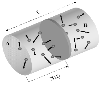
Figure 1: The adiabatic piston: an insulating cylinder divided into two regions by a movable, frictionless and insulating piston.

The relevant variable of the system is the position $x(t)$ of the moving wall with respect to its central position $L/2$, the harmonic potential being not prescribed but naturally emerging, as well as the friction term, as the result of the internal dynamics of the system.

We recall that the adiabatic-piston problem deals with a system consisting (see Fig.1) of an adiabatic cylinder of length $L$, divided into two sections A and B, containing the same number $n$ of gas moles in different equilibrium states, by a fixed frictionless adiabatic piston . At a given instant t=0, the piston is let free to move and the problem is to predict the final equilibrium state of the system. This deceivingly simple question, which cannot be actually answered in the frame of equilibrium thermodynamics, has been firstly solved in 1996 in the frame of a simple kinetic model Crosignani96 and has since then given rise to a number of papers of increasing sophistication. Both analytic Piasecki99 ; Chernov02 ; Munakata01 ; Gruber03 and molecular dynamics approaches Kestemont00 ; Renne01 ; White02 ; Mansour05 reveal the existence of two successive stages of evolution, the first one leading the system to a state of mechanical equilibrium (where the pressures in both sections are equal) and the second, intrinsically random and occurring over a much longer time scale, to a final state of both mechanical and thermal equilibrium (where the average position of the piston is equal to L/2 and the average gas temperatures in the two sections become equal). The above conclusions have been basically drawn by investigating the average behavior of the significant variables describing the system evolution but less attention has been devoted to the fluctuations around these average quantities, which are somehow assumed to be small. By extending and clarifying the results of a previous paper Crosignani01 , we wish to show how this is not always the case. More precisely, if one starts from specific initial conditions, then for spatial dimensions of the cylinder corresponding to the mesoscopic range (about 1 micron) and for values of the ratio $\mu=M/M_{g}$ between the piston and the gas mass lesser than one, fluctuations around equilibrium position can be a sizeable fraction of the average quantities, larger by a factor $\sqrt{M/m}$ ($m$ being the mass of the single gas molecule) than the ones expected if the system were in thermal equilibrium. This makes rather questionable the statement that in this case a final equilibrium configuration can be actually reached. Actually, the evolution of the system from an initial state in which both $x(t)=X(t)-L/2$ and $\dot{x}(t)$ are zero and the temperatures are equal in the two sections exhibits unexpected features: the system fails to settle down to a well-defined equilibrium state since the piston never comes to a stop but keeps wandering symmetrically around the initial position,performing oscillations whose mean-square value (evaluated over an ensemble of many replica) is much larger than that pertaining to standard thermal fluctuations. According to this behavior, the system appears to deserve the name of perpetuum mobile, even if there is no preferential direction of motion ($\langle x\rangle=\langle\dot{x}\rangle=0$). This unusual behavior can be associated with a possible challenge to the Second Law. In fact, a suitable process can be conceived through which the entropy of the isolated adiabatic piston system turns out to undergo a significant decrease (see Sections IV-V). In practice, as we shall see below, no significant entropy decrease occurs outside a mesoscopic regime corresponding to spatial dimensions of a few microns; in fact, the time interval $t_{as}$ over which the significant entropy decrease occurs depends on the fourth power of $L$ ($t_{as}\propto L^{4}$): thus, any deviation from the above spatial scale gives rise to such large $t_{as}$ as to affect the validity of our model. We note that the coincidence between the spatial scales over which the model is valid and a typical biological dimension is definitely intriguing.

II The stochastic adiabatic piston

The investigations of the adiabatic-piston dynamics appeared in the last ten years (see, e.g., Crosignani96 ; Piasecki99 ; Chernov02 ; Munakata01 ; Gruber03 ) have placed into evidence two distinct stages of temporal evolution. The first one occurs, on a relatively short time scale, when the system is let free to evolve from an initial configuration in which the two sections are in thermal equilibrium at different pressures, and leads to a final mechanical equilibrium (equal pressures) configuration that depends on the initial conditions. The second one is characterized by a stochastic dynamic evolution during which the common pressure on the two sides remains essentially constant, and may eventually lead to a final equilibrium configuration in which also the temperatures attain a common value and the piston is in the central position. In this section, we confine ourselves to the second stage by investigating the piston dynamics starting from a specific initial configuration characterized by $x(t=0)=\dot{x}(t=0)=0$ and by a common temperature $T_{0}$ in the two sections. In particular, we wish to focus our attention on the fluctuations of the piston positions around $L/2$. In effect, while $\langle x(t)\rangle$ and $\langle\dot{x}(t)\rangle$ turn out to vanish at all times, as a priori dictated by symmetry, there is a range of values of the system parameters, corresponding to a mesoscopic regime where the mean-square value $\langle x^{2}(t)\rangle^{1/2}$ can be a not negligible fraction of the piston half-length $L/2$, a quite surprising result which seems to indicate that no effective final equilibrium position can be reached.

We start from the equation describing the deterministic piston motion in the presence of a finite pressure difference, that is Crosignani96

$$\ddot{X}=\displaystyle\frac{nR}{M}\left(\frac{T_{A}}{X}-\frac{T_{B}}{L-X}\right)-\sqrt{\frac{8nRM_{g}}{\pi M^{2}}}\left(\frac{\displaystyle\sqrt{T_{A}}}{X}+\frac{\displaystyle\sqrt{T_{B}}}{L-X}\right)\dot{X}+\frac{M_{g}}{M}\left(\frac{1}{X}-\frac{1}{L-X}\right)\dot{X}^{2}$$ (1)

where $R$,$M_{g}$ and $M$ are the molar gas constant, the common values of the gas masses in $A$ and $B$, and the piston mass, respectively, while the dot stands for derivation with respect to time. It has been derived by assuming that the velocity distributions of the ideal gas in the two sections are Maxwellian, i.e., that thermal equilibrium is continuously restored on a time scale much shorter than the characteristic time scale of the piston motion, an assumption which has to be checked a posteriori. We observe that Eq.(1) is identical to the one obtained by Munakata and Ogawa (Eq. (22)of Ref. Munakata01 )but for the extra-term containing $\dot{X}^{2}$. This term, which is negligible for finite pressure-difference in the two sides, turns out to play a fundamental role when studying the piston dynamics for equal pressures, i.e., in the situation investigated in the present paper. In this case, Eq.(1) has to be suitably modified. In effect, besides setting equal to zero the first term on its R.H.S. associated with pressure difference, we have to explicitly take into account the random nature of the hits suffered by the piston because of the collisions with the gas molecules. To this aim, we resort to Langevin’s approach (see, e.g. Crosignani01 ) based on the introduction of an ad hoc Langevin acceleration $a(t)$, so that Eq.(1) is superseded by

$$\ddot{X}=-\frac{N}{M}\sqrt{\frac{8km}{\pi}}\left(\frac{\displaystyle\sqrt{T_{A}}}{X}+\frac{\displaystyle\sqrt{T_{B}}}{L-X}\right)\dot{X}+\frac{Nm}{M}\left(\frac{1}{X}-\frac{1}{L-X}\right)\dot{X}^{2}+a(t)\text{,}$$ (2)

where $k$ is the Boltzmann constant and $N=M_{g}/m$ is the number of molecules of mass $m$ on each side.

By taking again advantage of the equal pressure condition, i.e., $T_{A}(t)/X(t)=T_{B}(t)/[L-X(t)]=2T_{0}/L$ Eq.(2) can be rewritten as

$$\ddot{X}+\frac{4N}{N}\sqrt{\frac{kT_{0}m}{\pi L}}\left(\frac{1}{\sqrt{X}}+\frac{1}{\sqrt{L-X}}\right)\dot{X}+\frac{2Nm}{M}\left[\frac{X-L/2}{X(L-X)}\right]\dot{X}^{2}=a(t)\text{.}$$ (3)

Determining the correct expression for $a(t)$ is a delicate task since the standard Langevin approach does not in general carry over to nonlinear dynamical systems VanKampenBook , as the one described by Eq.(3). In order to be able to take advantage of the Langevin method, we linearize the above equation: a) by considering small displacements around the starting position of the piston, that is $|(X-L/2)|/(L/2)<<1$ and b) by approximating the square $\dot{X}^{2}$ of the piston velocity by the average thermal value $kT_{0}/M$ ; both hypotheses have to be proved consistent a posteriori. More precisely, by resorting to assumption b) and by using Langevin’s method , it is possible to identify two characteristic times, $t_{th}$ and $t_{as}>>t_{th}$ (see Eq.(10)). The first one represents the temporal scale over which the piston velocity thermalizes, while the second one is the characteristic time over which the large piston-position fluctuations occur. The relation $t_{th}<<t_{as}$ justifies a posteriori the application of the fluctuation-dissipation theorem.

After introducing the new variable $x(t)=X(t)-L/2$, the linearized version of Eq.(3) reads

$$\ddot{x}+\frac{4N}{\sqrt{\pi}}\frac{v_{0}}{L}\left(\frac{m}{M}\right)\dot{x}+4N\frac{v_{0}^{2}}{L^{2}}\left(\frac{m}{M}\right)^{2}x=a(t)\text{,}$$ (4)

$v_{0}=(2kT_{0}/m)^{1/2}$ being the most probable velocity of the corresponding gas Maxwellian distribution. SommerfeldBook At this point, a straightforward application of the fluctuation-dissipation theorem Pathria yields

$$\langle a(t)a(t^{\prime})\rangle=\frac{16N}{\sqrt{\pi}L}v_{0}^{3}\left(\frac{m}{M}\right)^{2}\delta(t-t^{\prime})\text{.}$$ (5)

According to the above results, the variable $x(t)$, describing the evolution of the state of our system, obeys an equation formally similar to that of a “Brownian particle” in one dimension. However, the potential term and the viscous drag have naturally emerged out of the internal dynamics of the system and do not correspond to an external active force or to a phenomenological friction term as in the case of Brownian motors. If we define

$$\beta=\frac{4N}{\sqrt{\pi}}\frac{v_{0}}{L}\frac{m}{M}\text{,}\hskip 28.45274pt\omega^{2}=4N\frac{v_{0}^{2}}{L^{2}}\left(\frac{m}{M}\right)^{2}$$ (6)

Eq.(4) is formally identical to that describing the Brownian motion of a harmonically-bound particle of mass $M$, that is

$$\ddot{x}+\beta\dot{x}+\omega^{2}x=a(t)$$ (7)

where $a(t)$ is the Langevin acceleration, a case which has been thoroughly investigated in the literature Chandrasekhar43 .

III The piston as a harmonically-bound Brownian particle

The solution of the stochastic differential equation (7) governing the piston motion is readily obtained in terms of the general results provided in Chandrasekhar43 for the Brownian motion of a harmonically-bound particle. Equation (7),together with Eq.(6), describe an “overdamped” case (in fact, $\beta/\omega=\sqrt{16/\pi}\sqrt{N}>>1$, since $N$ is typically a large number).For this situation, one has Chandrasekhar43

$$\begin{array}[]{l}\langle x(t)\rangle=x_{0}e^{-\beta t/2}\left(\cosh\frac{\beta_{1}t}{2}+\frac{\beta}{\beta_{1}}\sinh\frac{\beta_{1}t}{2}\right)+\frac{2u_{0}}{\beta_{1}}e^{-\beta t/2}\sinh\frac{\beta_{1}t}{2}\text{,}\\ \langle u(t)\rangle=u_{0}e^{-\beta t/2}\left(\cosh\frac{\beta_{1}t}{2}-\frac{\beta}{\beta_{1}}\sinh\frac{\beta_{1}t}{2}\right)-\frac{2x_{0}\omega^{2}}{\beta_{1}}e^{-\beta t/2}\sinh\frac{\beta_{1}t}{2}\text{,}\\ \langle x(t)^{2}\rangle=\langle x(t)\rangle^{2}+\frac{kT_{0}}{M\omega^{2}}\left[1-e^{-\beta t}\left(2\frac{\beta^{2}}{\beta_{1}^{2}}\sinh^{2}\frac{\beta_{1}t}{2}+\frac{\beta}{\beta_{1}}\sinh\beta_{1}t+1\right)\right]\text{,}\\ \langle u(t)^{2}\rangle=\langle u(t)\rangle^{2}+\frac{kT_{0}}{M}\left[1-e^{-\beta t}\left(2\frac{\beta^{2}}{\beta_{1}^{2}}\sinh^{2}\frac{\beta_{1}t}{2}-\frac{\beta}{\beta_{1}}\sinh\beta_{1}t+1\right)\right]\text{,}\end{array}$$ (8)

where $u(t)=dx/dt$ , $x_{0}=x(t=0)$, $u_{0}=u(t=0)$ and

$$\beta_{1}=\sqrt{\beta^{2}-4\omega^{2}}\cong\beta-2\omega^{2}/\beta\text{.}$$ (9)

In our case $x_{0}=0$, $u_{0}=0$, so that, as expected, $\langle x\rangle=\langle u\rangle=0$ at all times (see Eqs. (8)_1,2). By taking the temporal asymptotic limit of the above equations, it is possible to recognize the existence of two characteristic time scales $t_{th}$ and $t_{as}$ , such that $t_{th}<<t_{as}$, given by

$$\begin{array}[]{l}t_{th}=\frac{1}{2\beta}\text{,}\\ t_{as}=\frac{\beta}{2\omega^{2}}\text{.}\end{array}$$ (10)

They respectively represent the time over which the piston velocity thermalizes, i.e., its mean-square attains the value

$$\langle\dot{x}^{2}\rangle_{as}=\frac{kT_{0}}{M}\text{,}$$ (11)

and the time over which the mean-square value of the piston position reaches the asymptotic value

$$\langle x^{2}\rangle_{as}=\frac{kT_{0}}{M\omega^{2}}\text{.}$$ (12)

By using Eq.(6) we have

$$t_{as}=\frac{1}{2\sqrt{\pi}}\frac{L}{v_{0}}\frac{M}{m}=\frac{1}{2\sqrt{\pi}}\frac{L}{v_{0}}N\mu$$ (13)

and

$$t_{th}=\frac{\pi}{4N}t_{as}.$$ (14)

Since $N>>1$, the asymptotic time $t_{as}$ is much larger than the thermalization time $t_{th}$, which justifies the replacement in Eq.(3) of $\dot{X}^{2}$ with its thermal value given by Eq.(11). It is worth noting that the difference between the time scales of $\langle x^{2}\rangle$ and $\langle\dot{x}^{2}\rangle$ (i.e. $t_{as}>>t_{th}$) is associated with the presence of the sign “plus” and “minus” in the r.h.s. of Eq. (8)₃ and (8)₄, respectively. In fact, it is the minus sign in Eq. (8)₄ which is responsible for the cancellation of the slowly-decaying asymptotic terms in $\langle u^{2}\rangle$, while these terms, present in Eq. (8)₃, dictate the long time behavior of $\langle x^{2}\rangle_{as}$.

The asymptotic mean-square displacement $\langle x^{2}\rangle_{as}$ of the piston from its central equilibrium position $x=0$ is, according to Eqs. (8) and (6),

$$\langle x^{2}\rangle_{as}=\frac{\mu}{2}\left(\frac{L}{2}\right)^{2}=\frac{1}{2N}\frac{M}{m}\left(\frac{L}{2}\right)^{2}\text{.}$$ (15)

In the limit $\mu<<1$ (that is, small piston mass with respect to gas mass), the root-mean square displacement $\langle x^{2}\rangle_{as}^{1/2}$ is much smaller than $L/2$, so that both assumptions justifying the linearization of Eq.(7), and thus the application of Langevin’s approach, are verified. These fluctuations can be compared with those pertaining to a diathermal piston, associated with a system identical with the one described above but for the presence of a thermally conducting piston instead of an adiabatic one. To this end, let us assume the piston in Fig.1 to be a good heat conductor, so that both sections possess the common constant temperature $T_{0}$. Any displacement $x$ of the piston from the central position results in an unbalance $p(x)$ between the pressures $p_{A}(x)$ and $p_{B}(x)$ in the two sections, i.e.,

$$\Delta p(x)=p_{A}(x)-p_{B}(x)=\frac{NkT_{0}}{\mathcal{A}(L/2+x)}-\frac{NkT_{0}}{\mathcal{A}(L/2-x)}\text{,}$$ (16)

where $\mathcal{A}$ is the transverse section area, so that the force $F(x)$ exerted by the gas on the piston reads

$$F(x)=\frac{NkT_{0}}{L/2+x}-\frac{NkT_{0}}{L/2-x}\cong-\frac{2NkT_{0}}{(L/2)^{2}}x\text{,}$$ (17)

having assumed $|x|<<L/2$, as verified a posteriori. Therefore, the piston feels both the thermal bath at temperature $T_{0}$ and the harmonic potential

$$V(x)=\frac{NkT_{0}}{(L/2)^{2}}x^{2}\text{,}$$ (18)

and, as a consequence, its position probability-density $P(x)$ reads

$$P(x)=\sqrt{\frac{N}{\pi(L/2)^{2}}}\exp\left[-\frac{N}{(L/2)^{2}}x^{2}\right]\text{.}$$ (19)

The associated mean square value $\langle x^{2}\rangle$ is

$$\langle x^{2}\rangle=\frac{1}{2N}\left(\frac{L}{2}\right)^{2}\text{,}$$ (20)

smaller than the corresponding mean square displacement of the adiabatic piston (see Eq.(15)) by a factor $m/M$. Note that Eq.(20) agrees with the standard result obtained in the frame of equilibrium-thermodynamic microscopic fluctuations. NewCallen

Our derivation clarifies the basic difference between adiabatic and diathermal situation. In the first case, the restoring force acting on the piston is given by $-(8NkT_{0}m/L^{2}M)x$ (see Eq.(4)), while, in the second it reads $-(8NkT_{0}/L^{2})x$ (see Eq.(17)), so that the restoring force acting on the adiabatic piston is $m/M$ times smaller than that acting on the diathermal one. We stress that the anomalously large fluctuations of the adiabatic piston are not limited to the macroscopic regime, but are also present in the mesoscopic regime, provided the number of molecules $N$ is large enough, as in our case, to justify the use of ordinary concepts of pressure and temperature. This accounts for the peculiarity of the adiabatic piston system. The large random displacements of the piston are not trivially related to the system dimensions, but to its adiabatic nature: the diathermal piston exhibits a mean-square-value $\langle x^{2}\rangle=(m/M)\langle x^{2}\rangle_{as}$ (see Eq.(20) and Eq.(15)) smaller by a factor $m/M$ than the corresponding factor for the adiabatic piston.

IV Variation of the entropy

The peculiar behavior of the adiabatic-piston system discussed above has a natural counterpart in its entropy variations. In order to clarify this point, we note that the entropy behavior of our system is not uniquely defined. First, let us consider an ensemble of identical systems, in each of which the piston is let indefinitely free to move starting from the central position $x=0$ at time $t=0$. After a time interval reasonably larger than $t_{as}$, the probability distribution of the piston position will stay unchanged. Accordingly, it is possible to define an entropy of the system (gas+piston) ensemble whose value turns out to be larger than the initial one pertaining to the one in which all pistons are fixed in the central position. The above entropy does not allow for a simple statistical interpretation like Boltzmann’s one. The latter requires a single system in thermal equilibrium, and this is not the case for the wandering adiabatic piston. Thus, to give meaning to Boltzmann’s entropy, we consider a single system and stop the piston either at a given time of the order of $t_{as}$ or at a given prefixed position of the order $\langle x^{2}\rangle_{as}^{1/2}$. The two procedures are conceptually quite different. In fact, halting the piston at a given time requires a device comparable in size with the piston-position fluctuations it is trying to harness: in other words, the stopping mechanism seems to behave like a demon device while it rectifies the large piston fluctuations, thus forbidding any violation of the Second Law. Similar arguments go back to Smoluchowsky (see ref. Smolu ), and an interesting example is connected with the Feynman’s pawl and ratchet device. FeynmanBook Vice versa, in principle, if the halting device is placed at a position $\bar{x}$ chosen a priori (e.g., $\bar{x}=+\langle x^{2}\rangle_{as}^{1/2}$), the piston stopping operation takes place without the intervention of relevant statistical fluctuations, i.e., without any demon mechanism. Of course, due to the random nature of the piston wandering, we do not know when the halting process will take place. However, if we wait long enough (e.g., for a time of the order of a few $t_{as}$), there is a high likelihood that the piston has come to a halt at the prefixed position. The above argument highlights a peculiar feature of the adiabatic piston system. Unlike other systems in which unusually large thermal fluctuations cannot be rectified without introducing comparable external fluctuations, the piston wandering can be conveniently exploited. If the piston is stopped at a prefixed position, the Boltzmann gas entropy significantly decreases without any entropy increase of the environment. To clarify this point, we consider the entropy change $\Delta S$ undergone by the system when passing from the equilibrium state in which the piston is held in the central position to the final one in which the piston is stopped at the position $x=\bar{x}$. Recalling that the pressure does not change during the process (see Sect.II), we have

$$\Delta S=\Delta S_{A}+\Delta S_{B}=nc_{p}\ln\frac{L/2+\bar{x}}{L/2}+nc_{p}\ln\frac{L/2-\bar{x}}{L/2}=nc_{p}\ln\left[1-\left(\frac{\bar{x}}{L/2}\right)^{2}\right]$$ (21)

where $c_{p}$ is the molar heat at constant pressure and $n$ the common number of molecules in sections A and B. By recalling Eq.(15) and that $\bar{x}^{2}/(L/2)^{2}=\langle x^{2}\rangle_{as}/(L/2)^{2}$ is a small number, Eq. (21) yields

$$\frac{\Delta S}{k}=\frac{nc_{p}}{k}\ln\left[1-\left(\frac{\bar{x}}{L/2}\right)^{2}\right]\cong-\frac{nc_{p}}{k}\left(\frac{\bar{x}}{L/2}\right)^{2}=-\frac{c_{p}}{2R}N\mu\text{,}$$ (22)

or, by comparing it with the standard entropy fluctuations $\Delta S_{th}=(knc_{p})^{1/2}$ Landau

$$\frac{\Delta S}{\Delta S_{th}}=-\frac{1}{2}\sqrt{\frac{c_{p}}{R}}\sqrt{N}\mu\text{.}$$ (23)

This corresponds, whenever $\mu\sqrt{N}>>1$, i.e. $M/m>>\sqrt{N}$, to a sensible negative entropy decrease, and constitutes a violation of the Second Law, consistent with the perpetuum mobile behavior of the system. In particular, if the system is embedded in a thermal bath at temperature $T_{0}$, it is possible to devise a cyclic process by means of which the work

$$W\cong kT_{0}N\mu$$ (24)

can be extracted from the environment (see Appendix). Actually, according to the accumulated experimental evidence confirming the validity of the Second Law, we do not expect these results to hold true in standard macroscopic situations. In fact, our model imposes strict limitations on the spatial scale over which our results can be trusted. In order to assess these limitations, we refer to the specific case of a gas at standard conditions of temperature and pressure. In this case, expressing hereafter $L$ in microns, and assuming the volume of the piston to be $L^{3}$, $N=3\times 10^{7}L^{3}$ it follows from Eq.(23) that

$$\frac{\Delta S}{\Delta S_{th}}=-5\times 10^{3}L^{3/2}\mu\text{,}$$ (25)

while from Eq.(13) we have, taking $v_{0}=4\times 10^{8}$ microns/sec (molecular oxygen),

$$t_{as}=5\times 10^{-2}\mu L^{4}\text{sec.}$$ (26)

We now observe that, if we reasonably require the work $W$ extracted in a cycle to scale with the system dimensions, i.e., with $N$, the factor $\mu$ has to be kept constant when varying the system dimensions. Therefore, Eq. (26) reveals an extremely sensitive fourth-power dependence of $t_{as}$ on the linear dimension of the system, which severely limits the applicability of our model to values of $L$ up to a few microns. In fact, beyond this mesoscopic scale, $t_{as}$ becomes so large as to invalidate our results. As an example, for $\mu=0.01$ and $L=1cm$, one gets $t_{as}=5\times 10^{12}sec$, that is about 1000 centuries! Conversely, by taking $L=1\mu m$, we get for $t_{as}$ a reasonable value of $5\times 10^{-4}$ sec, while $\Delta S/\Delta S_{th}=-50$ is still quite large. It is important to stress that this specific mesoscopic regime, around $1\mu m$, has emerged spontaneously from the adiabatic-piston problem, without the introduction of any ad hoc parameter. The Second Law, stating that the entropy of an isolated system cannot decrease, is actually violated in the specific example provided above. The associated spatial scale appears to set a borderline between the macroscopic realm and the mesoscopic one.

Figure 2: Normalized asymptotic standard deviation $\eta$ of the piston position as a function of $\mu$ and $N=3\times 10^{4}$ (averaged over 1000 realizations). The continuous line represents the predicted behavior in the linearized regime (see Eq. (15)).

V Beyond the linear regime

The above approach has allowed us to deal with the situation $\mu\ll 1$. In order to have an insight into the behavior of our process in the more general case $\mu\lesssim 1$, we assume Langevin’s approach to be approximately valid also in this moderately nonlinear regime, and use the nonlinear Eq.(3) with the same stochastic acceleration $a(t)$ worked out in the linear case. After introducing the dimensionless units $\xi=X/L$ and $\tau=t/t_{o}$, where $t_{o}=4\sqrt{2}t_{th}$, Eq.(3) reads

$$\frac{d^{2}\xi}{d\tau^{2}}+\left(\frac{1}{\sqrt{\xi}}+\frac{1}{\sqrt{1-\xi}}\right)\frac{d\xi}{d\tau}-\frac{1}{\mu}\left(\frac{1}{\xi}-\frac{1}{1-\xi}\right)\left(\frac{d\xi}{d\tau}\right)^{2}=\sigma\alpha(\tau),$$ (27)

where $a(\tau)$ is a unitary-power white noise process and $\sigma^{2}=(\pi/2\sqrt{2})(\mu/N)$. This last equation can be numerically integrated by adopting a second-order leap-frog algorithm as the one developed in reference Qiang00 .

In particular, we can evaluate the asymptotic value of the mean-square root deviation $\eta\equiv\langle(\xi-1/2)^{2}\rangle^{1/2}$ as a function of $\mu$ and, for a given value of $\mu$ , the time evolution of $\langle\left(d\xi/d\tau\right)^{2}\rangle$. Fig.2 shows that the asymptotic mean-square root displacement of the piston increases as $\sqrt{\mu}$ for $\mu\lesssim 0.3$ , in fairly good agreement with the linearized theory (see Eq.(15)), while it tends to saturate for larger values of $\mu$. Fig. 3 confirms that the piston velocity attains its thermal value in a time much shorter than the asymptotic time $t_{as}$, a necessary condition for the application of Langevin’s approach. As far as the entropy change $\Delta S$ is concerned, the linear dependence on $\bar{x}^{2}=\langle x^{2}\rangle_{as}$ predicted by Eq.(22) implies as well its saturation for increasing $\mu$ . The above results show that, for fixed N, both piston asymptotic displacement and entropy decrease saturate with increasing piston mass $M$.

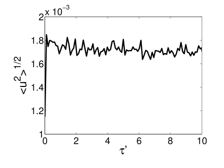
Figure 3: Time evolution of the r.m.s. of the normalized piston velocity $u=d\xi/d\tau$ as a function of $\tau^{\prime}=10^{-4}t/t_{0}$, for $\mu=0.5$ and $N=3\times 10^{4}$, averaged over $1000$ realizations.

VI Conclusions

In the present paper, we have examined the dynamic evolution of the adiabatic piston system starting from both mechanical and thermal equilibrium. Obviously, in this case $\langle x\rangle=0$ and $\langle\dot{x}\rangle=0$ for symmetry reasons, so that the significant quantity is $\langle x^{2}(t)\rangle^{1/2}$. This situation can be analyzed by generalizing the deterministic kinetic model developed in Crosignani96 with the introduction of Langevin’s force. The resulting equation for $x(t)$ turns out to be, whenever the mass $M$ of the piston is small compared to the gas mass $M_{g}$, completely identical to that describing the Brownian motion of an harmonically-bound particle of mass $M$. This allows us to provide an analytic expression for $\langle x^{2}(t)\rangle^{1/2}$ , which can be a sizeable fraction of the cylinder length $L$ (see Eq. (15)), thus implying that the piston never reaches an equilibrium position but keeps oscillating around its initial position $x=0$. This peculiar behavior is restricted to systems possessing specific spatial dimensions pertaining to a mesoscopic realm, where the laws of thermodynamics are not necessarily valid. The fact that the piston never stops is strictly related to the finite length of the cylinder: if we allow the length $L$ of the cylinder to go to infinity (as assumed, for example, in Gruber03 ), the ratio $M/M_{g}$ goes to zero and so does $\langle x(t)^{2}\rangle^{1/2}/(L/2)$ (see Eq.(15)). At the same time, $t_{as}$ becomes extremely large, so that, in this limit, the piston practically does not move. In view of this, the violation of the Second Law does not appear that startling since it concerns a regime outside the macroscopic thermodynamic limit. However, it can be interpreted as the signature of something remarkable happening at the borderline between the macroscopic and mesoscopic realms, signaling that a new way of looking at standard thermodynamic concepts may be needed if we wish to continue to apply them outside the boundaries within which they were first introduced.

In order to have an insight into the regime of mild nonlinearity occurring when $\mu=M/M_{g}$ approaches unity, we have numerically solved the stochastic Eq.(27) with the standard initial conditions adopted in our model. The results of the linearized approach are in good agreement with those associated with the numerical solution of Eq.(27).

The same problem of time evolution and approach to equilibrium of the system has been also considered by using molecular dynamics simulations.Kestemont00 ; Renne01 ; White02 ; Mansour05 These typically involve a considerable number of point particles (around $500$) which model the gas inside the cylinder and are separated by a frictionless movable piston, without internal degrees of freedom, against which they undergo perfectly elastic collisions. Some general features emerge from the numerical analysis, which reveal, consistently with our results, a very slow approach to the final equilibrium state.

In particular, Ref White02 presents the molecular dynamics simulations of a system evolving from an initial state in which the piston is fixed and the number of particles and the temperatures in both sections are equal, which is precisely the case we are dealing with in the present paper. Our analytic approach predicts a relaxation time (see Eq.(13)) which, in the normalized units adopted in White02 ($v_{0}=2$, $m=1$ and $L=60$), reads $t_{as}=(30/\sqrt{\pi})(M/m)\cong 17M$. This is in remarkably good agreement with the molecular dynamics simulations reported in White02 (see Fig.5 of Ref.White02 ) where, for $M<100$ (corresponding to $\mu=M/N=100/250=0.4$), $t_{as}=16M$.

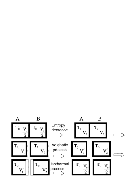
Figure 4: Cyclic process through which work can be extracted from a thermal bath at temperature $T_{0}$.

In conclusion, our simple kinetic analytic description has revealed that Callen’s adiabatic piston can exhibit, when starting from a particular mechanical and thermal equilibrium state, large fluctuations, a very intriguing feature which presents the characteristics of perpetuum mobile. This occurs for very specific spatial dimensions of the system (around $1\mu m$), pertaining to the mesoscopic regime. Whether this is actually challenging the limits of validity of the Second Law seems a legitimate question, whose answer may shed some light on the understanding of small-scale nonequilibrium devices.

We wish to thank Noel Corngold for his constant encouragement and many useful comments.

Appendix

If our system is embedded in a thermal bath at temperature $T_{0}$ and pressure $P_{0}$, the following process, sketched in Fig. 4 , can be used for extracting work from the environment. In the first panel, the system is in the initial state. The second panel shows the system after the entropy decrease $\Delta S$ has occurred. At this point, we separate the two sections (panel 3) and drive the two gases back to the initial temperature $T_{0}$ by means of two reversible adiabatic processes, the relation between the new volumes $V^{\prime}_{1}$ and $V^{\prime}_{2}$ and the previous volumes $V_{1}$ ,$V_{2}$ and temperatures $T_{1}$,$T_{2}$ being

$$V^{\prime}_{1}=V_{1}(T_{1}/T_{0})^{\frac{1}{\gamma-1}}\text{,}\hskip 28.45274ptV^{\prime}_{2}=V_{2}(T_{2}/T_{0})^{\frac{1}{\gamma-1}}\text{.}$$ (28)

This is followed (panel 4) by two reversible isothermal processes in which the two sections are in contact with the thermal bath at temperature $T_{0}$, which take the two sections back to the initial temperature $T_{0}$ and volume $V_{0}/2$ (frame 5). The total work extracted in the process is

$$W=W_{1}+W_{2}=nRT_{0}\ln(\frac{V_{0}}{V^{\prime}_{1}})+nRT_{0}\ln(\frac{V_{0}}{V^{\prime}_{2}})=nRT_{0}\ln[\frac{V_{0}^{2}(T_{0}^{2})^{\frac{1}{\gamma-1}}}{V_{1}V_{2}(T_{1}T_{2})^{\frac{1}{\gamma-1}}}]\text{.}$$ (29)

Since $V_{1}+V_{2}=2V_{0}$ and $T_{1}+T_{2}=2T_{0}$, we obviously have $T_{0}^{2}>T_{1}T_{2}$ and $V_{0}^{2}>V_{1}V_{2}$, so that a work $W$ larger than zero has been obtained at the expenses of the heat $Q=W$ extracted by a single source (the thermal bath). It can be easily checked that $W=-T_{0}\Delta S\cong kT_{0}N\mu$, that is each gas molecule contributes with a fraction $\mu kT_{0}/2$ to the work extracted in the process.

References

- (1) H. B. Callen, Thermodynamics (Wiley, New York, 1960), p. 321.
- (2) E. Schroedinger, What is life? (Cambridge University Press, Cambridge, 1945), Ch. VI.
- (3) R. Reinmann and P. Hanggi, Appl.Phys. A 175, 169. (2002).
- (4) R. P. Feynman, R. Leighton, and M. Sands, The Feynman Lectures on Physics I (Addison-Wesley, Reading, Mass, 1965), ch. 39.
- (5) B. Crosignani, P. Di Porto, and M. Segev, Am. J. Phys. 64, 610 (1996).
- (6) J. Piasecki and Ch. Gruber, Physica A 264, 463 (1999).
- (7) N. I. Chernov, J. L. Lebowitz and Sinai Ya. G., Russian Mathemathical Surveys 57, 1045 (2002).
- (8) T. Munakata and H. Ogawa, Phys. Rev. E 64, 036119 (2001).
- (9) Ch. Gruber, S. Pache and A. Lesne, J. Stat. Phys. 112, 1177 (2003).
- (10) E. Kestemont, C. Van den Broeck, and M. Malek Mansour, Europhys. Lett. 49, 143 (2000).
- (11) M. Renne, M. Ruijgrok, and T. Ruijgrok, Acta Physica Polonica 32, 4183 (2001).
- (12) J. A. White, F. L. Roman, A. Gonzalez, and S. Velasco, Europhys. Lett. 59, 479 (2002).
- (13) M. Malek Mansour, C. Van den Broeck, and E. Kestemont, Europhys. Lett. 69, 510 (2005).
- (14) B. Crosignani and P. Di Porto, Europhys. Lett. 53, 290 (2001).
- (15) N. Van Kampen N, Stochastic Process in Physics and Chemistry (North-Holland, Amsterdam, 1992).
- (16) A. Sommerfeld, Thermodynamics and Statistical Mechanics (Academic Press, New York, 1956), p. 177.
- (17) See, e.g., R. K. Pathria, Statistical Mechanics, 2nd ed. (Buttherworth-Heineman, Oxford,1996), p. 481.
- (18) See, e.g., S. Chandrasekhar, Rev. Mod. Phys. 15, 1 (1943).
- (19) H. B. Callen, Thermodynamics and an Introduction to Thermostatistics (Wiley, New York, 1985, second edition), pag. 428.
- (20) M. Smoluchowski, Phys. Zeit. 12, 1069 (1912).
- (21) L. Landau and E. Lifshitz, Statistical Physics (Pergamon Press, Oxford) 1969.
- (22) J. Qiang and S. Habib, Phys. Rev. E62, 7430 (2000).