Numerical study of dynamo action at low magnetic Prandtl numbers

Abstract

We present a three–pronged numerical approach to the dynamo problem at low magnetic Prandtl numbers $P_{M}$. The difficulty of resolving a large range of scales is circumvented by combining Direct Numerical Simulations, a Lagrangian-averaged model, and Large-Eddy Simulations (LES). The flow is generated by the Taylor-Green forcing; it combines a well defined structure at large scales and turbulent fluctuations at small scales. Our main findings are: (i) dynamos are observed from $P_{M}=1$ down to $P_{M}=10^{-2}$; (ii) the critical magnetic Reynolds number increases sharply with $P_{M}^{-1}$ as turbulence sets in and then saturates; (iii) in the linear growth phase, the most unstable magnetic modes move to small scales as $P_{M}$ is decreased and a Kazantsev $k^{3/2}$ spectrum develops; then the dynamo grows at large scales and modifies the turbulent velocity fluctuations.

The generation of magnetic fields in celestial bodies occurs in media for which the viscosity $\nu$ and the magnetic diffusivity $\eta$ are vastly different. For example, in the interstellar medium the magnetic Prandtl number $P_{M}=\nu/\eta$ has been estimated to be as large as $10^{14}$, whereas in stars such as the Sun and for planets such as the Earth, it can be very low ($P_{M}<10^{-5}$, the value for the Earth’s iron core). Similarly in liquid breeder reactors and in laboratory experiments in liquid metals, $P_{M}\ll 1$. At the same time, the Reynolds number $R_{V}=UL/\nu$ ($U$ is the r.m.s. velocity, $L$ is the integral scale of the flow) is very large, and the flow is highly complex and turbulent, with prevailing non-linear effects rendering the problem difficult to address. If in the smallest scales of astrophysical objects plasma effects may prevail, the large scales are adequately described by the equations of magnetohydrodynamics (MHD),

$$\frac{\partial{\bf v}}{\partial t}+{\bf v}\cdot\nabla{\bf v}=-\nabla{\cal P}+\mathbf{j}\times\mathbf{B}+\nu\nabla^{2}\mathbf{v}+{\bf F}$$ (1)

$$\frac{\partial{\bf B}}{\partial t}+{\bf v}\cdot\nabla{\bf B}=\mathbf{B}\cdot\nabla{\bf v}+\eta\nabla^{2}{\bf B}\ ,$$ (2)

together with ${\bf\nabla}\cdot{\bf v}=0$, $\nabla\cdot{\bf B}=0$, and assuming a constant mass density. Here, $\mathbf{v}$ is the velocity field normalized to the r.m.s. fluid flow speed, and $\mathbf{B}$ the magnetic field converted to velocity units by means of an equivalent Alfvén speed. ${\cal P}$ is the pressure and $\mathbf{j}=\nabla\times\mathbf{B}$ the current density. ${\bf F}$ is a forcing term, responsible for the generation of the flow (buoyancy and Coriolis in planets, mechanical drive in experiments).

Several mechanisms have been studied for dynamo action, both analytically and numerically, involving in particular the role of helicity moffat (i.e. the correlation between velocity and its curl, the vorticity) for dynamo growth at scales larger than that of the velocity, and the role of chaotic fields for small-scale growth of magnetic excitation (for a recent review, see axel ). Granted that the stretching and folding of magnetic field lines by velocity gradients overcome dissipation, dynamo action takes place above a critical magnetic Reynolds number $R_{M}^{c}$, with $R_{M}=P_{M}R_{V}=UL/\eta$. Dynamo experiments engineering constrained helical flows of liquid sodium have been successful KarlsruherigaGailitisStefaniTilgner . However, these experimental setups do not allow for a complete investigation of the dynamical regime, and many groups have searched to implement unconstrained dynamos GydroSpecialIssue . Two difficulties arise: first, turbulence now becomes fully developed with velocity fluctuations reaching up to 40% of the mean; second, it is difficult to engineer flows with helical small scales so that the net effect of turbulence is uncertain. Recent Direct Numerical Simulations (DNS) address the case of randomly forced, non-helical flows with magnetic Prandtl numbers from 1 to 0.1. Contradictory results are obtained: it is shown in alex04 that dynamo action can be inhibited for $P_{M}<1/4$, while it is observed in axel that the dynamo threshold increases as $P_{M}^{-1/2}$ down to $P_{M}\sim 0.3$. Experiments made in von Kármán geometries (either spherical or cylindrical) have reached $R_{M}$ values up to 60 pefbour . Also, MHD turbulence at low $P_{M}$ has been studied in the idealized context of turbulent closures kn67 . In this context, turbulent dynamos are found, and the dependences of $R_{M}^{c}$ upon three quantities are studied, namely $P_{M}$, the relative rate of helicity injection, and the forcing scale. An increase of $\sim 20\%$ in $R_{M}^{c}$ is observed as $P_{M}$ decreases from 1 to $\sim 3\times 10^{-5}$. Recently, the Kazantsev-Kraichnan kazan model of $\delta$-correlated velocity fluctuations has been used to study the effect of turbulence. It is shown that the threshold increases with the rugosity of the flow field dario02 , and that turbulence can either increase or decrease the dynamo threshold depending on the fine structure of the velocity fluctuations leprovost .

There is therefore a strong motivation to study how the dynamo threshold varies as $P_{M}$ is progressively decreased, for a given flow. In this letter we focus on a situation where the flow forcing is not random, but generates a well defined geometry at large scales, with turbulence developing naturally at small scales as the $R_{V}$ increases. This situation complements recent numerical works alex04 ; axel ; dario02 ; leprovost and is quite relevant for planetary and laboratory flows. Specifically, we consider the swirling flow resulting from the Taylor-Green forcing meb :

$${{\bf F}_{\rm TG}(k_{0})}={2F}\,\left[\begin{array}[]{c}\sin(k_{0}~{}x)\cos(k_{0}~{}y)\cos(k_{0}~{}z)\\ -\cos(k_{0}~{}x)\sin(k_{0}~{}y)\cos(k_{0}~{}z)\\ 0\end{array}\right]\ ,$$ (3)

with $k_{0}=2$, so that dynamo action is free to develop at scales larger or smaller than the forcing scale $k_{f}=k_{0}\sqrt{3}$. This force generates flow cells that have locally differential rotation and helicity, two key ingredients for dynamo action moffat ; axel . Note that the net helicity, i.e. averaged in time and space, is zero in the $2\pi$-periodic domain. However strong local fluctuations of helicity are always present in the flow. Small scales are statistically non-helical. The resulting flow also shares similarities with the Maryland, Cadarache and Wisconsin sodium experiments GydroSpecialIssue , and it has motivated several numerical studies at $P_{M}\sim 1$ NoreDuddleyJames ; MarieBourgoin .

code	$N$	$R_{V}$	$L$	$R_{M}^{c}$	$1/P_{M}^{c}$	$k_{\rm MAX}$	$k_{D}$	$\rho$
DNS	$64$	30.5	2.15	28.8	1.06	2	5	-7.2
DNS	$64$	40.5	2.02	31.7	1.28	2	5	-6.3
DNS	$64$	128	1.9	62.5	2.05	4	9	-3.5
DNS	$128$	275	1.63	107.9	2.55	5	11	-2.15
DNS	$256$	675	1.35	226.4	2.98	7	21	$\sim-5/3$
DNS	$512$	874.3	1.31	192.6	4.54	9	26	$\sim-5/3$
LAMHD	$64$	280	1.68	117.3	2.38	6	11	-2.25
LAMHD	$128$	678.3	1.35	256.6	2.64	8	12	$\sim-5/3$
LAMHD	$128$	880.6	1.32	242.1	3.64	9	22	$\sim-5/3$
LAMHD	$256$	1301.1	1.3	249.3	5.22	9	31	$\sim-5/3$
LAMHD	$512$	3052.3	1.22	276.4	11.05	10	45	$\sim-5/3$
LES	$128$	2236.3	1.37	151.9	14.72	5	21	$-5/3$
LES	$256$	5439.2	1.39	141	38.57	5	31	$-5/3$
LES	$512$	12550	1.42	154.6	81.19	5	40	$-5/3$

Table 1: Parameters of the computation: code used, linear grid resolution $N$, Reynolds number $R_{V}$, integral length scale $L$ (defined from the kinetic energy spectrum $L=2\pi\int{k^{-1}E_{V}(k)dk}/\int{E_{V}(k)dk}$), critical magnetic Reynolds number $R_{M}^{c}$, inverse magnetic Prandtl number $1/P_{M}^{c}$, wavenumber $k_{\rm MAX}$ with the largest magnetic energy, characteristic wavenumber $k_{D}$ of magnetic field gradients (defined as the maximum of the current density spectrum), and kinetic spectral index $\rho$ in the range $[k_{\rm MAX},k_{D}]$. The values of $\rho$, $L$ and $U$ used in the definitions of the Reynolds and magnetic Prandtl numbers, are computed as time averages during the steady state of the hydrodynamic simulation; $k_{MAX}$ and $k_{D}$ are computed as time averages during the linear regime of the dynamo simulation closest to $R_{M}^{c}$.

Figure 1: $R_{M}^{c}$ for dynamo action versus inverse $P_{M}$. Symbols are: $\times$ (DNS), $+$ (LAMHD), and $\diamond$ (LES). Transverse lines indicate error bars in the determination of $R_{M}^{c}$, as the distance between growing and decaying runs at a constant $R_{V}$.

Our numerical study begins with DNS in a 3D periodic domain. The code uses a pseudo-spectral algorithm, an explicit second order Runge-Kutta advance in time, and a classical dealiasing rule — the last resolved wavenumber is $k=N/3$ where $N$ is the number of grid points per dimension. Resolutions from $64^{3}$ to $512^{3}$ grid points are used, to cover $P_{M}$ from 1 to $1/5$. However, DNS are limited in the Reynolds numbers and the (lowest) $P_{M}$ they can reach. We then use a second method, the LAMHD (or $\alpha$) model, in which we integrate the Lagrangian-averaged MHD equations LAMHD ; mmp04 . This formulation leads to a drastic reduction in the degrees of freedom at small scales by the introduction of smoothing lengths $\alpha_{V}$ and $\alpha_{M}$. The fields are written as the sum of filtered (smoothed) and fluctuating components: $\mathbf{v}=\mathbf{u_{s}}+\delta\mathbf{v}$, $\mathbf{B}=\mathbf{B_{s}}+\delta\mathbf{B}$, with $\mathbf{u_{s}}=G_{\alpha_{V}}\otimes\mathbf{v}$, $\mathbf{B_{s}}=G_{\alpha_{M}}\otimes\mathbf{B}$, where ‘$\otimes$’ stands for convolution and $G_{\alpha}$ is the smoothing kernel at scale $\alpha$, $G_{\alpha}({\bf r},t)=\exp[-r/\alpha]/4\pi\alpha^{2}r$. Inversely, the rough fields can be written in terms of their filtered counterparts as: $\mathbf{v}=(1-\alpha_{V}^{2}\nabla^{2})\ \mathbf{u_{s}}$ and $\mathbf{B}=(1-\alpha_{M}^{2}\nabla^{2})\ \mathbf{B_{s}}$. In the resulting equations, the velocity and magnetic field are smoothed, but not the fields’ sources, i.e. the vorticity and the current density mp02 . This model has been checked in the fluid case against experiments and DNS of the Navier-Stokes equations in 3D CFHOTW99 , as well as in MHD in 2D mmp04 . Finally, in order to reach still lower $P_{M}$, we implement an LES model. LES are commonly used and well tested in fluid dynamics against laboratory experiments and DNS in a variety of flow configurations parviz , but their extension to MHD is still in its infancy (see however LESMHD ). We use a scheme as introduced in ppp04 , aimed at integrating the primitive MHD equations with a turbulent velocity field all the way down to the magnetic diffusion with no modeling in the induction equation but with the help of a dynamical eddy viscosity  CL81 :

$$\nu(k,t)=0.27[1+3.58(k/K_{c})^{8}]\sqrt{E_{V}(K_{c},t)/K_{c}}\ ;$$ (4)

$K_{c}$ is the cut-off wavenumber of the velocity field, and $E_{V}(k,t)$ is the one-dimensional kinetic energy spectrum. A consistency condition for our approach is that the magnetic field fluctuations be fully resolved when $2\pi/K_{c}$ is smaller than the magnetic diffusive scale $\ell_{\eta}\sim L/R_{M}^{3/4}$.

The numerical methods, parameters of the runs, and associated characteristic quantities are given in Table I. In all cases, we first perform a hydrodynamic run, lasting about 10 turnover times, to obtain a statistically steady flow. Then we add a seed magnetic field, and monitor the growth of the magnetic energy $E_{M}$ for a time that depends on the run resolution; it is of the order of 1 magnetic diffusion time $\tau_{\eta}=(2\pi)^{2}/\eta$ at $64^{3}$, but it drops down to $\tau_{\eta}/5$ at $512^{3}$. We define the magnetic energy growth rate as $\sigma=d\log E_{M}/dt$, computed in the linear regime ($t$ is in units of large scale turnover time). The dynamo threshold corresponds to $\sigma=0$. For each configuration (Table I), we make several MHD simulations with different $P_{M}$, varying $\eta$, and for a fixed $R_{V}$ defined by the hydrodynamic run. We bound the marginal growth between clearly decaying and growing evolutions of the magnetic energy. This procedure is unavoidable because of the critical slowing down near threshold.

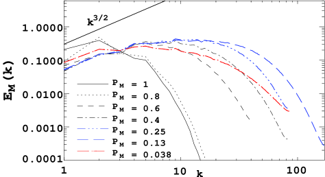
Figure 2: Magnetic spectra for $P_{M}=1$ to $P_{M}=0.4$ (DNS), $P_{M}=0.25,0.13$ (LAMHD), $P_{M}=0.038$ (LES), at a time within the linear growth of magnetic energy.

At $P_{M}=1$, the dynamo self-generates at $R_{M}^{c}=30$. As $P_{M}$ is lowered, we observe in the DNS that the threshold reaches $R_{M}^{c}=70$ at $P_{M}=0.5$ and then increases steeply to $R_{M}^{c}=226$ at $P_{M}=0.3$; at lower $P_{M}$ it does not increase anymore, but drops slightly to a value of 200 at $P_{M}=0.2$ (Fig.1 and Table I). We then continue with LAMHD simulations to reach lower $P_{M}$. To ensure the consistency of the method, we have run overlapping DNS and LAMHD simulations in the range from $P_{M}=0.4-0.2$, the agreement of the two methods being evaluated by the matching of the magnetic energy growth (or decay) rates for identical $(P_{M},R_{M})$ parameters. We have observed that a good agreement between the two methods can be reached if one uses two different filtering scales $\alpha_{V}$ and $\alpha_{M}$ in LAMHD, chosen to maintain a dimensional relationship between the magnetic and kinetic dissipation scales, namely $\alpha_{V}/\alpha_{M}=P_{M}^{3/4}$. Our observation with the LAMHD computations is that the steep increase in $R_{M}^{c}$ to a value over 250 is being followed by a plateau for $P_{M}$ values down to 0.09. We do note a small but systematic trend of the LAMHD simulations to overestimate the threshold compared to DNS. We attribute it to the increased turbulent intermittency generated by the $\alpha$ model, but further investigations are required to describe fully this effect. The LES simulations allow us to further our investigation; with this model the threshold for dynamo self-generation remains constant, of the order of 150, for $P_{M}$ between $10^{-1}$ and $10^{-2}$.

In regards to the generation of dynamo action in the Taylor-Green geometry we thus find: (i) at all $P_{M}$ investigated a dynamo threshold exists; (ii) as $P_{M}$ drops below 0.2 - 0.3, the critical $R_{M}^{c}$ levels and remains of the order of 200; (iii) the steep initial increase in $R_{M}^{c}$ is identified with the development of an inertial range in the spectra of kinetic energy. As the kinetic energy spectrum grows progressively into a Kolmogorov $k^{-5/3}$ spectrum, $R_{M}^{c}$ ceases to have significant changes – cf. Table 1.

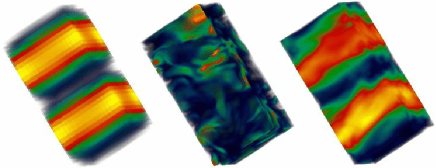
Figure 3: Spatial distributions of the magnetic energy for two Taylor-Green cells (DNS) : $P_{M}=1$, $R_{V}\sim 30$ at $t=20$ (left), $P_{M}=0.4$, $R_{V}=675$ at $t=20$ (center), and $t=150$ (right).

We plot in Fig. 2 the magnetic energy spectra $E_{M}(k)$ during the linear growth phase, at identical instants when normalized by the growth rate. Four features are noteworthy: first, the dynamo grows from a broad range of modes; second, the maximum of $E_{M}(k)$ moves progressively to smaller scales as $P_{M}$ decreases, a result already found numerically in axel ; third, a self-similar magnetic spectrum, $E_{M}(k)\sim k^{3/2}$, develops at the beginning during the linear growth phase — as predicted by Kazantsev kazan and found in other numerical simulations of dynamo generation by turbulent fluctuations axel ; alex04 . This is a feature that thus persists when the flow has well defined mean geometry in addition to turbulence. Lastly we observe that the initial magnetic growth at small scales is always followed by a second phase where the magnetic field grows in the (large) scales of the Taylor-Green flow. Figure 3 shows renderings of the magnetic energy and compare low and high Reynolds number cases. When the dynamo is generated at low Reynolds number ($R_{V}\sim 30$ and $P_{M}=1$), the magnetic field is smooth. As $P_{M}$ decreases and the dynamo grows from a turbulent field, one first observes a complex magnetic field pattern – for $t<40$, in the example shown in Fig.3(center). But as non-linear effects develop (here for times $t>40$) a large scale mode ($k=2$) dominates the growth with a structure that is similar to the one at low $R_{V}$. The initial growth of small scale magnetic fields and the subsequent transfer to a large scale dynamo mode is also clearly visible on the development in time of the magnetic and kinetic energies, in a high $R_{V}$ case, as shown in Fig. 4. During the linear growth, a wide interval of modes increase in a self-similar fashion, accounting for the complexity of the dynamo field - cf. Fig. 3(center). At a later time, the large scale field grows and the kinetic energy spectrum $E_{V}(k)$ is progressively modified at inertial scales. The spectral slope changes from a Kolmogorov $k^{-5/3}$ scaling to a steeper, close to $k^{-3}$, regime kmoins3 . The effect is to modify the turbulent scales and to favor the dynamo mode that is allowed by the large scale flow geometry. This is consistent with the development of a $k^{-5}$ magnetic spectrum, observed in the Karlsruhe dynamo experiment muller . It also corroborates the claim petrelis that the saturation of the turbulent dynamo starts with the back-reaction of the Lorentz force on the turbulent fluctuations.

Figure 4: Magnetic (thin line) and kinetic (thick line) spectra as a function of time at $P_{M}=0.4$ (DNS).

To conclude, using a combination of DNS, LAMHD modeling and LES, we show that, for the Taylor-Green flow forcing, there is a strong increase in the critical magnetic Reynolds number for dynamo action when $P_{M}$ is decreased, directly linked to the development of turbulence; and it is followed by a plateau on a large range of $P_{M}$ from $\sim 0.25$ to $\sim 10^{-2}$. In a situation with both a mean flow and turbulent fluctuations, we find that the selection of the dynamo mode results from a subtle interaction between the large and small scales.

Acknowledgements We thank D. Holm for discussions about the $\alpha$ model, and H. Tufo for providing computer time at UC-Boulder, NSF ARI grant CDA–9601817. NSF grants ATM–0327533 (Dartmouth) and CMG–0327888 (NCAR) are acknowledged. JFP, HP and YP thank CNRS Dynamo GdR, and INSU/PNST and PCMI Programs for support. Computer time was provided by NCAR, PSC, NERSC, and IDRIS (CNRS).

References

- (1) H.K. Moffatt. Magnetic Field Generation in Electrically Conducting Fluids, (Cambridge U.P., Cambridge, 1978).
- (2) A. Brandenburg and K. Subramanian, astro-ph/0405052, submitted to Phys. Rep. (2004).
- (3) A. Gailitis, Magnetohydrodynamics, 1, 63 (1996). A. Tilgner, Phys. Rev. A, 226, 75 (1997). R. Steglitz and U. Müller, Phys. Fluids, 13(3), 561 (2001). A. Gailitis, et al., Phys. Rev. Lett., 84, 4365 (2000).
- (4) See “MHD dynamo experiments”, special issue of Magnetohydodynamics, 38, (2002).
- (5) A. Schekochihin et al., New J. Physics 4, 84 (2002); A. Schekochihin et al. Phys. Rev. Lett. 92, 054502 (2004).
- (6) N.L. Peffley, A.B. Cawthrone, and D.P. Lathrop, Phys. Rev. E, 61, 5287 (2000). M. Bourgoin et al. Physics of Fluids, 14(9), 3046 (2001).
- (7) R.H. Kraichnan and S. Nagarajan, Phys. Fluids 10, 859 (1967); J. Léorat, A. Pouquet, and U. Frisch, J. Fluid Mech., 104, 419 (1981).
- (8) A.P. Kazantsev, Sov. Phys. JETP 26, 1031 (1968); R.H. Kraichnan, Phys. Fluids 11, 945 (1968).
- (9) S. Boldyrev and F. Cattaneo, Phys. Rev. Lett., 92, 144501 (2004); D. Vincenzi, J. Stat. Phys. 106, 1073 (2002).
- (10) N. Leprovost and B. Dubrulle, astro-ph/0404108, (2004).
- (11) M. Brachet, C. R. Acad. Sci. Paris 311, 775 (1990).
- (12) N.L. Dudley and R.W. James, Proc. Roy. Soc. Lond., A425, 407 (1989). C. Nore et al. Phys. Plasmas, 4,1 (1997).
- (13) L. Marié et al., Eur. J. Phys. B, 33, 469 (2003). M. Bourgoin et al., Phys. Fluids, 16, 2529 (2004).
- (14) D.D. Holm, Physica D 170, 253 (2002); Chaos 12, 518 (2002).
- (15) P.D. Mininni, D.C. Montgomery, and A. Pouquet , submitted to Phys. Fluids.
- (16) D.C. Montgomery and A. Pouquet, Phys. Fluids 14, 3365(2002).
- (17) S.Y. Chen et al., Phys. Fluids 11, 2343 (1999); S.Y. Chen et al., Physica D 133, 66 (1999).
- (18) R.S. Rogallo and P. Moin, Ann. Rev. Fluid Mech. 16, 99 (1984); C. Meneveau and J. Katz, Ann. Rev. Fluid Mech. 32, 1 (2000).
- (19) A. Pouquet, J. Léorat, and U. Frisch, J. Fluid Mech., 77, 321 (1976); A. Yoshizawa, Phys. Fluids 30, 1089 (1987); M. Theobald, P. Fox, and S. Sofia, Phys. Plasmas 1, 3016 (1994); W-C. Müller and D. Carati, Phys. Plasmas 9, 824 (2002). B. Knaepen and P. Moin, Phys. Fluids, 16, 1255, (2004).
- (20) Y. Ponty, H. Politano, and J.F. Pinton, Phys. Rev. Lett. 92, 144503 (2004).
- (21) J.P. Chollet and M. Lesieur, J. Atmos. Sci. 38, 2747 (1981).
- (22) A. Alemany et al., J. Méca. 18, 277 (1979).
- (23) U. Müller, R. Stieglitz, and S. Horanyi, J. Fluid Mech., 498, 31 (2004)
- (24) F. Pétrélis and S. Fauve, Eur. Phys. J. B, 22, 273 (2001).