Low-energy excitations of a linearly Jahn-Teller coupled orbital quintet.

Abstract

The low-energy spectra of the single-mode $h\otimes(G+H)$ linear Jahn-Teller model is studied by means of exact diagonalization. Both eigenenergies and photoemission spectral intensities are computed. These spectra are useful to understand the vibronic dynamics of icosahedral clusters with partly filled orbital quintet molecular shells, for example C₆₀ positive ions.

I Introduction

In icosahedral molecules and ions, there occurs the possibility of a partial occupancy of a quintet of orbitally degenerate electronic levels, of $h$ symmetry. A notable example is that of positive C₆₀ ions, with one (or several) holes in a $h_{u}$ molecular orbital Lueders03 ; Bohme99 . At the adiabatic level, partly occupied quintet states are unstable against molecular distortions involving the vibrational modes of the molecule. Distortions along nondegenerate $A$ modes do not involve symmetry reduction, are therefore not of Jahn-Teller (JT) type, and can be trivially treated as phonon shifts: thus we will ignore $A$ modes altogether. Distortions involving fourfold-degenerate $G$ and fivefold-degenerate $H$ modes reduce the molecular symmetry, and are responsible for the leading (linear) contribution to the splitting of the fivefold molecular level. Other ($T_{1}$ and $T_{2}$) modes are involved in higher-order couplings, which become dominating only for substantially large distortions. Under specific circumstances (null or very strong linear coupling) the inclusion of higher-order couplings could become essential. However, the present work follows the standard practice of neglecting all higher-then-linear coupling terms and treating the phonons as harmonic oscillators Ceulemans ; CeulemansII . This approximation provides a simplified model meant to capture the basic shape of the five adiabatic potential energy surfaces (APES) in a neighborhood of their high-symmetry conical intersection, hopefully extending out to include the JT minima. The advantage of the idealized linear model is that it involves a minimal number of parameters, and that it can therefore be studied in detail, drawing fairly general conclusions, applicable to a wide enough range of realistic systems.

Indeed, besides C₆₀, orbital quintets could be relevant for the spectroscopy of other icosahedral molecules and clusters among those synthesized in recent years, including smaller and higher fullerenes such as C₂₀ and C₈₀, B₁₂ or B₈₄ clusters, B₁₂H₁₂, the smallest icosahedral systems Si₁₃, Na₁₃, or Mg₁₃, and icosahedral structures with 13, 19, 55, and 147 atoms in xenon clusters. With different coupling patterns possibly realized in those different systems, it is of clear interest to investigate how the vibronic spectrum changes as a function of electron-vibration coupling. For simplicity, here we restrict ourselves to a single mode (of either $G$ or $H$ type) coupled to the orbital quintet.

Several works Ceulemans ; CeulemansII ; Szopa attach the JT problem of the orbital quintet in the linear approximation and for a single mode. These early works are mainly studies of the APES, and in particular of its minima, with the phonon coordinates treated as classical variables. Other papers deal with the full quantum mechanical problem, and provide either approximate Moate96 ; Moate97 ; Polinger03 or exact Delos96 ; hbyh solutions, sometimes for the many-modes case Manini03 ; ManyModes . The quantum mechanical dynamics of the entangled electron-phonon system is affected by an electronic geometric phase, whose presence/absence has relevant consequences, in particular, for the ground-state (GS) symmetry AMT ; Delos96 ; Paris97 ; Polinger03 ; Koizumi99 ; Lijnen03 , thus for magnetic resonance spectroscopies Abragam . In particular, Ref. hbyh, provides a detailed study of the evolution of the tunneling splitting through the range of coupling parameters for an $H$ mode.

Unfortunately, to date, no experimental determination of the tunneling splitting in any icosahedral JT system is available. In contrast, spectroscopic techniques can and do provide direct measurements of the JT vibronic spectrum. For example, molecular photoemission Bruhwiler97 ; Canton02 was recently shown Manini03 to provide relatively detailed information on the low-lying part of the vibronic spectrum of C${}_{60}^{+}$, especially in a specific symmetry sector ManiniComm03 . A clean theoretical understanding of the general features of this vibronic spectrum is therefore desirable.

The present work provides precisely an exact determination of the low-lying vibronic levels of the single-mode linear model, those usually of most direct experimental access. The spectrum is studied through a wide range of coupling parameters, from weak to strong coupling. In practice, the reported results are mainly relevant for weak to intermediate coupling, since, as noted above, the linear JT model is little more than a mathematical curiosity in the strong-coupling limit, where higher-than-linear powers of the distortion become dominant. The vibronic spectra presented in this work illustrate several interesting quantum phenomena characteristic of dynamical JT. Several numerical energies reported in Appendix A can be used as benchmarks of the accuracy of future calculations based on approximate approaches, for example of the type of Refs. Moate96, ; Dunn03, .

II Model and calculation

The model CeulemansII ; hbyh ; Moate96 describing the JT coupling of the orbitally degenerate $h$ quintet with the molecular vibrations of symmetry $\Lambda=G,\,H$ is conveniently formulated as follows hbyh ; Manini01 ; Lueders02 :

$$\hat{H} = \hat{H}_{0}+\hat{H}_{\rm vib}+\hat{H}_{\rm e-v}\,,$$ (1)

$$\hat{H}_{0} = \epsilon\,\sum_{m\sigma}\hat{c}_{m\sigma}^{\dagger}\hat{c}_{m\sigma}\,,$$ (2)

$$\hat{H}_{\rm vib} = \frac{1}{2}\hbar\omega\sum_{\mu}\left(\hat{P}_{\mu}^{2}+\hat{Q}_{\mu}^{2}\right)\,,$$ (3)

$$\hat{H}_{\rm e-v} = \hbar\omega\,k^{\Lambda}\sum_{{r\sigma\,\mu mm^{\prime}}}g^{(r)}_{\Lambda}C^{r\Lambda\mu}_{m\;-m^{\prime}}\,\hat{Q}_{\mu}\,\hat{c}^{\dagger}_{m\sigma}\hat{c}_{m^{\prime}\sigma}\,.$$ (4)

Here $m$, $\mu$ label components within the degenerate multiplets, for example according to the $C_{5}$ character in the ${\cal I}\supset D_{5}\supset C_{5}$ group chain hbyh ; Butler81 , $C^{r\Lambda\mu}_{mm^{\prime}}$ are icosahedral Clebsch-Gordan coefficients Butler81 which couple two $h$ tensor operators and a $\Lambda$ tensor operator to a global scalar $A$ operator. $\hat{Q}_{\mu}$ are the dimensionless normal-mode vibrational coordinates (in units of the natural length scale of the harmonic oscillator), and $\hat{P}_{\mu}$ the corresponding conjugate momenta. The multiplicity $r=1,2$, needed for $\Lambda=H$ vibrations only, labels the two separate kinds of coupling allowed under the same symmetry Manini01 ; Butler81 : it represents the double occurrence of the $H$ representation in the direct product $h\times h$ (the icosahedral group is not simply reducible). Numerical factors $k^{G}=\frac{1}{4}{5^{\frac{1}{2}}}$, $k^{H}=\frac{1}{2}$ (which could otherwise be re-absorbed into the definition of $g_{\Lambda}$) are included to make contact with the notation of Ref. Manini01, .

Without any loss of generality, the energy position $\epsilon$ of the $h$ quintet will be taken as the zero of energy. In this single-mode problem, all energies are naturally measured in units of the vibrational quantum $\hbar\omega$. The second characteristic energy scale $g_{\Lambda}^{2}\hbar\omega$ (the JT energy) is smaller/larger than $\hbar\omega$ for small/large $g_{\Lambda}$ (weak/strong coupling). The weak-coupling regime is characterized by rapid tunneling among shallow clustered potential wells and strong non-adiabaticity associated to the vicinity to the conical intersection of the five Born-Oppenheimer potential sheets; the level structure is perturbatively related to the harmonic spectrum of $\hat{H}_{\rm vib}$. As the coupling grows to intermediate and strong, the JT wells deepen and move away from the conical intersection and from each other: tunneling decreases and the vibronic spectrum acquires a characteristically intricate structure, which simplifies again in the strong-coupling limit, where tunneling is exponentially suppressed and semiclassical considerations apply Polinger03 .

The adiabatic approximation, where the vibrational kinetic energy is neglected, provides the main (static JT) features of the strong-coupling limit. The distortion operators $\hat{Q}_{\mu}$ are treated as classical coordinates, and optimal distortions are obtained by minimizing the lowest APES Moate96 ; Moate97 , for example by means of the Öpik-Pryce method OP . These optimal distortions (JT wells, or minima) are associated to specific splitting patterns of the electronic quintet. In particular, $G$ modes produce a level pattern of the type $(-8,-3,-3,7,7)$, in correspondence to 10 JT wells of $D_{3}$ residual symmetry.

The situation is slightly more intricate for an $H$ mode CeulemansII ; hbyh ; Moate96 , due to the multiplicity $r=1,\,2$. The coupling scheme, associated to the $r\!=\!2$ Clebsch-Gordan coefficients, produces the splitting pattern $(-4,-1,-1,3,3)$ in correspondence to 10 $D_{3}$ minima, like the $G$ modes. The $r\!=\!1$ scheme produces a splitting pattern of the type $(-4,1,1,1,1)$, in correspondence to 6 JT minima of $D_{5}$ symmetry.

In practice, the two-scheme coupling for the $H$ modes is a convenient theoretical idealization, since any $H$ mode of a real molecule is associated to some amount of coupling of both $r\!=\!1$ and $r\!=\!2$ kind. This admixture is conveniently characterized by introducing two coupling constants for each $H$ mode, rather than one. The two dimensionless linear coupling parameters $g_{H}^{(1)}$, $g_{H}^{(2)}$ can be expressed in polar coordinates hbyh ; Manini01 as

$$g_{H}^{(1)}=g\,\cos\alpha\,,\qquad g_{H}^{(2)}=g\,\sin\alpha\,.$$ (5)

In summary, besides its frequency $\omega$, each $H$ vibrational mode is characterized by a pair ($g_{H}^{(1)}$, $g_{H}^{(2)}$) of linear couplings, or equivalently a global coupling intensity $g$ plus a mixing angle $\alpha$.

Figure 1: The splitting pattern of the electronic quintet in the $h\otimes H$ JT, as a function of the mixing angle $\alpha$. The lowest eigenvalue is nondegenerate, the two upper ones are both twofold degenerate; energies are in units of $g^{2}\hbar\omega$. At each value of $\alpha$, $Q$ is taken at the optimal classical distortion $Q_{\rm min}$.

Figure 1 shows the evolution of the quintet of electronic eigenvalues as $\alpha$ takes its possible values. Here, the molecular vibration operators are treated as classical variables, and are taken at the relevant static JT minimum, of $D_{5}$ or $D_{3}$ symmetry, appropriate for each value of $\alpha$. Pure coupling of type 1 is recovered at $\alpha\!=\!0$ and $\pi$, while pure coupling of type 2 occurs for $\alpha\!=\!\pi/2$. At the special angles $\alpha_{s}=\arctan(3/\sqrt{5})\simeq 0.296\,\pi\simeq 53.3^{\circ}$ and $\pi\!-\!\alpha_{s}$, where cusps occur in the $\alpha$-dependence of the eigenvalues, $D_{5}$ and $D_{3}$ minima are exactly degenerate: the JT minima collapse into a single flat trough, and the symmetry of the JT system is effectively larger than icosahedral CeulemansII ; Delos96 ; Paris97 ; noberry ; Judd84 ; Judd99 . Figure 1 shows that for a given coupling energy $g^{2}\hbar\omega$, the lowering of the lowest electronic state (equal twice the static JT energy gain) is strongest at $\alpha=0,\ \pi$ and weakest at $\alpha_{s},\ \pi\!-\!\alpha_{2}$.

To compute the exact vibronic spectrum of $\hat{H}$, full quantum-mechanical treatment must be applied also to the vibrational operators. The standard ladder-operator representation for the vibrational coordinates $\hat{Q}_{\mu}=\left(\hat{b}_{\mu}^{\dagger}+\hat{b}_{\mu}\right)/\sqrt{2}$ provides a natural product basis of harmonic phonon states centered on the undistorted geometry, times the electronic quintet. It is straightforward to write $\hat{H}$ matrix elements in this basis and diagonalize the resulting matrix. This basis centered on the high-symmetry point is especially convenient at weak coupling, where converged low-energy vibronic eigenenergies and eigenstates are obtained by including only few basis states. For large $g$, the number of basis states needed for a given accuracy of the low-energy levels grows rather quickly, approximately as $g^{2n_{\rm osc}}$, where $n_{\rm osc}=4$ for a $G$ mode and $n_{\rm osc}=5$ for an $H$ mode. For this reason, and because of the extreme sparseness of this problem, the Lanczos method of diagonalization Prelovsek00 ; Meyer89 is especially suitable here. We use a method very similar to the one employed in Ref. hbyh, , with the introduction of several refinements to deal with the problem of Lanczos ghost states, and the symmetry analysis. We check all results against basis truncation. For most results, inclusion of $n=35$ phonons in the basis is largely sufficient for an accuracy of $10^{-6}\hbar\omega$, but for occasional points in parameter space the basis needs to include up to $n=60$ phonons (over 8 million states) to guarantee the required accuracy. The spectra computed with this method and reported below draw a full quantitative link from weak through intermediate to strong coupling for the $h\otimes G$ and $h\otimes H$ linear dynamical JT model.

III Vibronic spectra: energies

III.1 The $h\otimes G$ JT

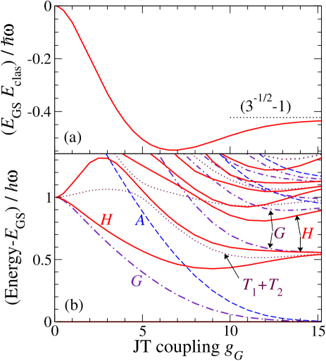
Figure 2: Exact vibronic spectrum of a single $G$ mode coupled to a $h$ level, as a function of the linear coupling parameter $g_{G}$. (a) GS energy, to which the adiabatic minimum lowering $E_{\rm clas}=\left(2-\frac{1}{18}g_{G}^{2}\right)\hbar\omega$ is subtracted. (b) Vibronic excitation energies (measured with respect to the GS). All levels are labeled according to their symmetry as $A$ (dashed), $T_{1}+T_{2}$ (dotted), $G$ (dot-dashed) and $H$ (solid).

Figure 2a shows the difference between the exact dynamical JT GS energy and $E_{\rm clas}$ (the classical adiabatic energy $-\frac{1}{18}g_{G}^{2}\hbar\omega$ of the 10 $D_{3}$ wells plus the zero-point energy $2\hbar\omega$ of the uncoupled oscillators), as a function of the coupling strength $g_{G}$ to a $G$ mode. This residual energy represents the part of JT energy gain not ascribable to trivial adiabatic lowering of the JT minima with respect to zero coupling: this energy difference gauges quantum-mechanical effects on the vibrational motion. The rapid decrease in GS energy at weak coupling is due to the large drop in quantum kinetic energy in the transition from harmonic oscillations around one isolated adiabatic minimum to rapid tunneling among 10 shallow minima. As these minima move apart, tunneling is suppressed, and the plotted energy difference turns back up to the strong-coupling value $(3^{-1/2}-1)\hbar\omega$, which measures the zero-point energy gain due to phonon softening at the anisotropic JT minima Lueders03 ; Leuven02 . Indeed, the second-order expansion of the lowest APES around any of the equivalent JT minima yields two normal modes (of symmetry $A_{1}$ and $A_{2}$ in the local $D_{3}$ group) both of frequency $\omega$, plus a twofold-degenerate softer mode (of symmetry $E$) of frequency $3^{-1/2}\omega$. The difference in harmonic zero-point energy $2\,\frac{1}{2}\hbar\omega+2\,\frac{1}{2}3^{-1/2}\hbar\omega-4\,\frac{1}{2}\hbar\omega=(3^{-1/2}-1)\hbar\omega$ provides an accurate estimate for the exact vibronic energy (Fig. 2a) at strong coupling, where inter-well tunneling is suppressed and the phonon dynamics reduces to harmonic oscillations around the JT wells. Note that the “new” frequencies at the wells are independent of the coupling strength $g_{G}$, since for different coupling $g_{G}$, the set of five APES differs only for a scaling factor, thus remaining self-similar. At weak coupling, the harmonic frequencies at the JT wells remain unchanged, but this expansion is practically irrelevant, since quantum kinetic energy delocalizes the motion far enough from the minima for anharmonic and nonadiabatic effects to dominate.

The vibronic GS symmetry remains $H$ at all couplings. This is eventually a consequence of a Berry phase of $\pi$ acquired by the electronic wavefunction as the distortions follow any of the cheapest (5-corner) loops through adjacent $D_{3}$ minima: this entanglement makes the totally symmetric $A$ vibronic combination of the wells less advantageous than the $H$ combination, which thus remains the GS for all $g_{G}$. Indeed, as seen in Fig. 2b, even at strong coupling, the $A$ vibronic state lies above both the $H$ GS and a $G$ excitation At strong coupling, these $5(H)+4(G)+1(A)$ states represent the 10 symmetry-adapted vibronic combinations of the harmonic GS’s at the 10 $D_{3}$ wells. Likewise, in the strong-coupling limit, higher excited states, represent suitably symmetrized combinations of vibrational excitations in the wells. In particular, the 20 states ($T_{1}+T_{2}+G+2\,H$) converging at strong coupling to $3^{-1/2}\hbar\omega$ represent the tunneling-symmetrized one-phonon oscillations of the new softer frequency. Similarly, the 20 states ($A+T_{1}+T_{2}+2\,G+H$) converging at strong coupling to $\hbar\omega$ represent the tunneling-symmetrized one-phonon oscillations of the modes at the original frequency $\hbar\omega$.

At weak coupling, the vibronic levels reconstruct the harmonic ladder, as expected when $\hat{H}_{\rm e-v}$ is a weak perturbation. The present exact calculation traces precisely the crossover from the weak to strong coupling regime: for accurate numeric eigenvalues, see Table 1 in the Appendix. It is worth noting that the lowest $A$ level, which at strong coupling is a low-energy tunneling excitation, correlates to the $2\,\hbar\omega$ multiplet at weak coupling Moate97 . Finally, note that the $T_{1}$ and $T_{2}$ levels are exactly degenerate for all values of the coupling.

III.2 The $h\otimes H$ JT

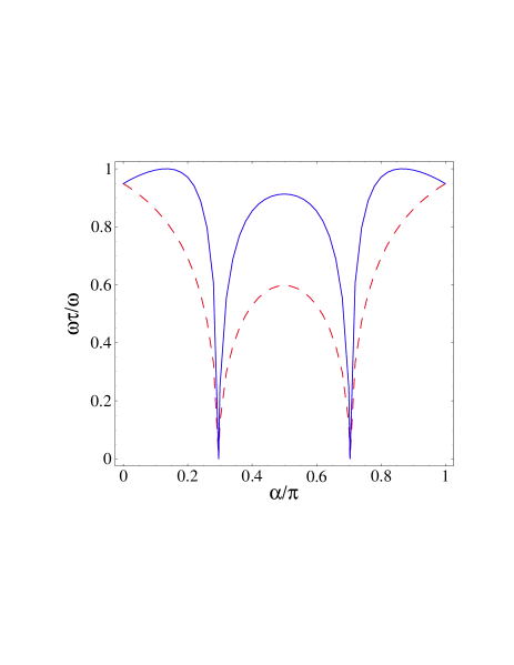
Figure 3: “Tangential” normal frequencies $\omega_{\tau}$ of vibration around the JT wells, in units of the original frequency $\omega$, as a function of $\alpha$. Both these modes are twofold degenerate. As customary of linear JT, the frequency of the fifth (radial) normal mode equals $\omega$, regardless of $\alpha$.

We move on now to study the spectrum for a vibrational mode of $H$ symmetry. The Hamiltonian $\hat{H}$ depends now on two parameters. Each vibronic eigenvalue traces a 2-dimensional surface as $g$ and $\alpha$ (or equivalently $g_{H}^{(1)}$ and $g_{H}^{(2)}$) are varied. The most effective presentation of these spectra is obtained by means of radial cuts at fixed $\alpha$, plus circular cuts at fixed $g$.

Like for the $G$ mode, the strong-coupling asymptotic vibronic energies, are determined by the normal frequencies of oscillation around the adiabatic JT minima, and these frequencies now depend on $\alpha$. The five normal modes separate into a radial vibration of unchanged frequency $\omega$ and symmetry $A_{1}$, plus two softer doubly-degenerate (of $E_{1}$ and $E_{2}$ symmetry for $D_{5}$ wells and both of $E$ symmetry for $D_{3}$ wells) tangential modes, represented in Fig. 3. For special $\alpha$ values, extra degeneracies occur:

• for $\alpha=0$ and $\pi$, the two tangential modes become degenerate at $\omega_{\tau}=(9/10)^{1/2}\omega$;

• for $\alpha\simeq 0.134\,\pi$ and $0.866\,\pi$, the upper tangential frequency tops at a maximum where it reaches the frequency $\omega$ of the radial mode;

• at the special $\alpha=\alpha_{s}$ and $\pi-\alpha_{s}$ points, both tangential frequencies vanish as the vibrations turn into free modes of pseudorotation along the flat JT trough;

• in addition, for $\alpha=\pi/2$, both soft modes reach a local maximum, of frequencies $\omega_{\tau}^{(1)}=(5/14)^{1/2}\omega$ and $\omega_{\tau}^{(2)}=(5/6)^{1/2}\omega$.

Observe that the normal frequencies at the wells only depend on $\alpha$, while they are independent of the coupling strength $g$, like for the $G$ mode. Again, these single-well harmonic frequencies determine the strong-coupling asymptotic vibronic energies, but they are essentially irrelevant at weak coupling, where inter-well tunneling dominates.

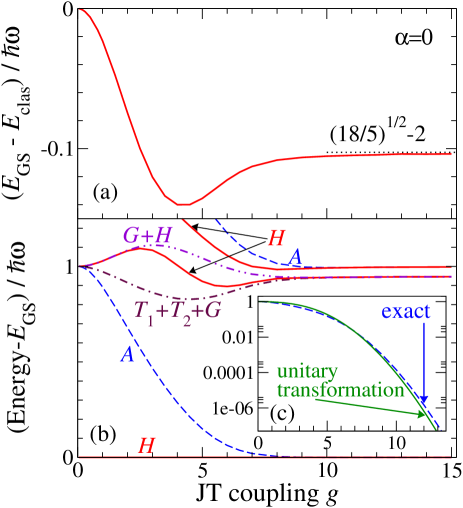
Figure 4: Exact vibronic spectrum of a single $H$ mode coupled to a $h$ level, as a function of the linear coupling parameter $g$, for $\alpha=0$. (a) GS energy, to which the energy of the adiabatic JT wells $E_{\rm clas}=\left(5/2-g^{2}/10\right)\hbar\omega$ is subtracted. (b) Vibronic excitation energies (measured with respect to the GS). The levels are labeled according to their icosahedral symmetry even though, for this special value of $\alpha$, the effective underlying symmetry is spherical. The conversion in spherical angular-momentum labels $[j]$ is $A\equiv[0]$, $H\equiv[2]$, $G+H\equiv[3]$, $T_{1}+T_{2}+G\equiv[1]+[3]$. (c) Comparison of the exact excitation energy of the lowest $A$ state (the tunneling splitting) with the approximate expression obtained in Ref. Moate97, by means of the unitary transformation method Bates87 .

Not unlike the $h\otimes G$ calculation, to draw the GS energy it is convenient to subtract the quantity

$$E_{\rm clas}(g,\alpha)=\left\{\!\!\begin{array}[]{ll}\left[\frac{5}{2}-\frac{1}{10}(\cos\alpha\;g)^{2}\right]\hbar\omega,&0\leq\alpha\leq\alpha_{s}\\ \\ \left[\frac{5}{2}-\frac{1}{18}(\sin\alpha\;g)^{2}\right]\hbar\omega,&\alpha_{s}\leq\alpha\leq\frac{\pi}{2}\\ \end{array}\right.\!\!\!.$$ (6)

$E_{\rm clas}(g,\alpha)$ represents the trivial zero-point energy $\frac{5}{2}\hbar\omega$ of $\hat{H}_{\rm vib}$ plus the adiabatic lowering of the $D_{5}$/$D_{3}$ JT well appropriate to that value of $\alpha$.

Figure 4a reports the exact GS energy, for the special mixing angle $\alpha=0$ (a mode of pure type $r=1$). This energy difference converges rapidly to its asymptotic value $[(18/5)^{1/2}-1]\hbar\omega$ at strong-coupling. Like for the $G$ mode, this is understood in terms of zero-point energy associated to the four frequencies $\omega_{\tau}=(9/10)^{1/2}\omega$ plus one frequency $\omega$ of the normal-mode vibrations at the JT minima.

The spectrum of excitations Fig. 4b is much less cluttered than that of the $G$ mode (Fig. 2b). The main reason is the larger than icosahedral effective symmetry of the Hamiltonian at this specific coupling angle. This larger (spherical) symmetry induces extra degeneracies among the vibronic levels, which one could in fact label with spherical angular-momentum labels. The lowest excited state is of $A$ symmetry: it is the one state which at strong coupling drops towards the $H$ GS. Together, these $5(H)+1(A)$ states represent the 6 symmetrized tunneling-split vibronic combinations of the harmonic GS’s at the 6 $D_{5}$ wells. An approximate analytical approach to this problem based on this idea (the unitary transformation method Bates87 ) yields Moate97 an estimate of the excitation energy (solid line in Fig. 4c): this approximation is seen to be fairly accurate throughout the range of couplings. The approximate expression underestimates the tunneling splitting at strong coupling due to the simplifying assumption of isotropic JT wells, of frequencies all equaling $\omega$, which therefore exaggerate the localization of the distorted states. Corrections due to the anisotropy of the wells were introduced in Ref. Dunn03, . In the Appendix, Table 2 reports a few of the vibronic eigenenergies used to draw Fig. 4.

Higher excitations cluster around the harmonic normal-mode energies at the $D_{5}$ wells: the tangential $\hbar\omega_{\tau}=(9/10)^{1/2}\hbar\omega$ and the radial $\hbar\omega$. The 24 states ($T_{1}+T_{2}+2G+2H$) around $\hbar\omega_{\tau}$ are symmetrized combinations of the four 1-phonon states per each of the six $D_{5}$ JT wells. Likewise, the 6 states ($H+A$) near $\hbar\omega$ are combinations of the 1-radial-phonon states in the $6$ wells. Note in particular that the two 1-phonon $H$ states remain almost degenerate until $g\lesssim 2$, they split significantly in the interval $2\lesssim g\lesssim 8$, and then re-converge again (to $\hbar\omega_{\tau}$) at strong coupling. At strong coupling, higher excitations (not drawn) are found in the overtone region $2\,\hbar\omega_{\tau}$, and above.

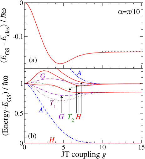
Figure 5: Exact vibronic spectrum of a single $H$ mode coupled to a $h$ level, as a function of the coupling parameter $g$, for $\alpha=\pi/10$. (a) GS energy, to which $E_{\rm clas}$ is subtracted. (b) Vibronic excitation energies measured with respect to the $H$ GS. All levels are labeled according to their symmetry as $A$ (dashed), $T_{1\,/\,2}$ (dotted), $G$ (dot-dashed) and $H$ (solid).

For $\alpha=\pi/10$, Fig. 5a shows the exact GS energy referred to $E_{\rm clas}$. This small value of $\alpha$ has little effect on the GS energy, as compared to the $\alpha=0$ case. On the contrary, the comparison of Fig. 5b with Fig. 4b shows that even such a small value of $\alpha$ (i.e. a tiny admixture of the coupling of type $r=2$) is sufficient to completely resolve the “accidental” degeneracies of the $\alpha=0$ spectrum. $A$ and $G$ states are little affected, while the $T_{1}$/$T_{2}$ degeneracy is widely broken. Likewise, the weak-coupling near degeneracy of the 1-phonon $H$ states for $\alpha=0$ is now widely split. Eventually, at strong coupling, these two $H$ states converge to different tangential frequencies of the JT wells.

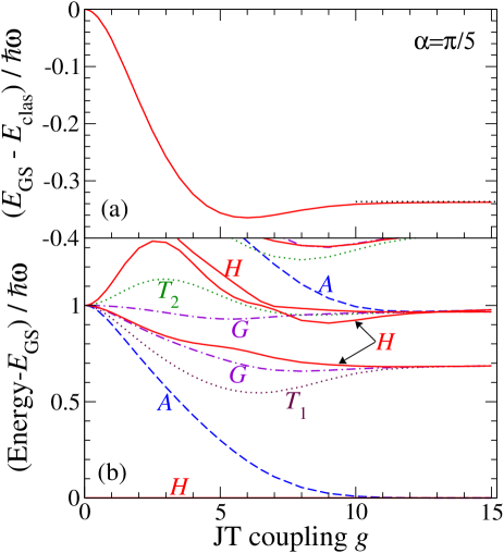
Figure 6: Same as Fig. 5 for $\alpha=\pi/5$.

Coming to the spectrum for $\alpha=\pi/5$, Fig. 6 shows a continuous evolution away from $\alpha=0$ through $\alpha=\pi/10$. We observe that, at strong coupling for both $\alpha=\pi/10$ and $\alpha=\pi/5$, only one new frequency is seen in the strong-coupling spectrum: that of decreasing $\omega_{\tau}$ for increasing $\alpha$ ($\omega_{\tau}=0.86\,\omega$ for $\alpha=\pi/10$, $\omega_{\tau}=0.69\,\omega$ for $\alpha=\pi/5$). Figure 3 confirms that the frequency $\omega_{\tau}$ of the other tangential mode is very close to its maximum $\omega$, thus very difficult to separate on this scale. In practice all 18 relevant one-phonon states converge near $\hbar\omega$ at strong coupling.

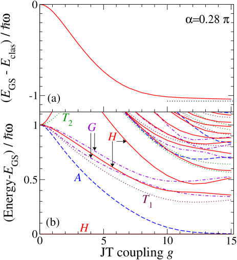
Figure 7: Same as Fig. 5 for $\alpha=0.28\,\pi\lesssim\alpha_{s}$.

Moving further away from this accidental degeneracy, to $\alpha=0.28\,\pi$ (Fig. 7), the two new tangential frequencies become $\omega_{\tau}^{(1)}\simeq 0.33\,\omega$ and $\omega_{\tau}^{(2)}\simeq 0.61\,\omega$. These frequencies are so small because of the nearness to the special angle $\alpha_{s}$ where $D_{5}$ and $D_{3}$ minima degenerate to a flat trough (see Fig. 3). These small values explain the twofold reason why the spectrum of Fig. 7b is so cluttered: (i) tunneling is only weakly suppressed by the low inter-well barriers, and (ii) several overtones and combinations of these soft tangential modes fit in the considered energy range. The large zero-point energy lowering shown in Fig. 7a is also well accounted for by the values of $\omega_{\tau}$.

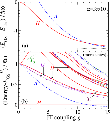
Figure 8: Exact vibronic spectrum of a single $H$ mode coupled to a $h$ level, as a function of $g$, for $\alpha=0.3\,\pi\gtrsim\alpha_{s}$. (a) GS energy, to which $E_{\rm clas}$ is subtracted; the GS is of $H$ symmetry at weak coupling, and of $A$ symmetry at strong coupling. (b) Vibronic excitation energies measured with respect to the lowest $H$ state.

The next point $\alpha=3\pi/10$ (Fig. 8) is located immediately beyond $\alpha_{s}$, with $D_{3}$ minima barely prevailing over $D_{5}$ distortions. Here, the tangential frequencies are as low as $\omega_{\tau}^{(1)}\simeq 0.125\,\omega$ and $\omega_{\tau}^{(2)}\simeq 0.247\,\omega$: this accounts for the huge zero-point energy lowering apparent in Fig. 8a in the strong-coupling limit. In contrast to all previous $\alpha$ values, where $D_{5}$ wells prevail, we observe here the celebrated Delos96 ; Moate96 ; hbyh level crossing (occurring at a rather strong coupling $g\simeq 12$) to a nondegenerate GS of $A$ symmetry. The vibronic spectrum (Fig. 8b) is now even more cluttered than for $\alpha=0.28\,\pi$, it shows an intricate pattern of level crossings (states of different symmetries) and avoided crossings (states of the same symmetry). Several higher-lying levels have been omitted in the plot for clarity. This is due to the exceedingly low normal frequencies at the wells, plus the larger number of wells (10 instead of 6). The clustering around the semiclassical frequencies is barely hinted, even for the rather strong coupling at the right side of the plot.

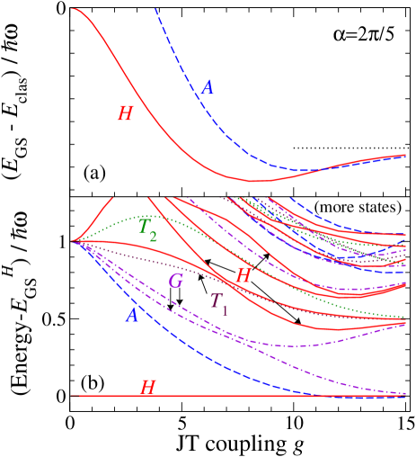
Figure 9: Same as Fig. 8, with $\alpha=2\pi/5$.

Coming now to $\alpha=2\pi/5$ (Fig. 9), the tangential frequencies at the $D_{3}$ minima are now $\omega_{\tau}^{(1)}\simeq 0.529\,\omega$ and $\omega_{\tau}^{(2)}\simeq 0.854\,\omega$, much larger than for the previous cut at $\alpha=3\pi/10$. These values account for the reduced zero-point energy lowering shown in Fig. 9a. Also, the spectrum (Fig. 9b) is less dense: the 10 tunneling states ($A+H+G$) converge to zero energy at strong coupling; the 20 1-phonon tangential states converging to $\hbar\omega_{\tau}^{(1)}$ are fairly well visible; the tangential $\hbar\omega_{\tau}^{(2)}$, radial $\hbar\omega$, and overtone $2\,\hbar\omega_{\tau}^{(1)}$ states are still substantially intermixed even at the large coupling of the right side of Fig. 9b. The splittings between $T_{1}$ and $T_{2}$ pairs are consistently reduced here, compared to previous values of $\alpha$. Note in particular that, in contrast to the $\alpha$ range producing $D_{5}$ wells, both 1-phonon $H$ states correlate at strong coupling to the lowest tangential mode of frequency $\hbar\omega_{\tau}^{(1)}$. A fairly general feature of the vibronic spectrum, especially visible in Figs. 2b, 9b, and 10b, is the rapid drop of several vibronic energies, then followed by a successive climb back at strong coupling where tunneling is suppressed and the motion gradually collapses to oscillations around the adiabatic wells.

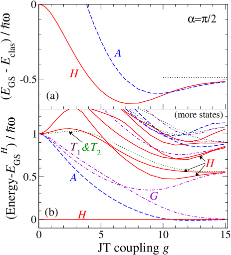
Figure 10: Same as Fig. 8, with $\alpha=\pi/2$.

At $\alpha=\pi/2$ (Fig. 10), JT coupling of pure $r=2$ type is acting. As illustrated in Fig. 3 above, the tangential frequencies at the JT wells reach here a local maximum $\omega_{\tau}^{(1)}\simeq 0.598\,\omega$ and $\omega_{\tau}^{(2)}\simeq 0.913\,\omega$. Accordingly, the zero-point energy lowering of Fig. 10a amounts to $[(5/14)^{1/2}+(5/6)^{1/2}-2]\hbar\omega=-0.490\,\hbar\omega$. The GS level crossing occurs now at a marginally smaller $g\simeq 10.7$, due to suppressed tunneling splitting. The spectrum is now even less dense than for previous values of $\alpha$, due to the larger frequencies at the JT wells, and the exact degeneracy of the $T_{1}$ and $T_{2}$ pairs. The 20 1-phonon tangential states ($G+2H+T_{1}+T_{2}$) converging to $\hbar\omega_{\tau}^{(1)}$ are well visible; the 20 states (of the same symmetries) converging to $\hbar\omega_{\tau}^{(2)}$ are still entangled with the 10 $\hbar\omega$ radial states ($A+H+T_{1}+T_{2}$).

For $\pi/2<\alpha\leq\pi$ the spectra are mirror symmetric around $\alpha=\pi/2$ to those reported for the interval $0\leq\alpha\leq\pi/2$. The only difference is that all $T_{1}$ and $T_{2}$ states (which always come in pairs) are exchanged.

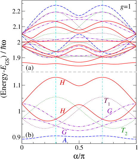
Figure 11: Exact vibronic spectrum of a single $H$ mode coupled to a $h$ electronic quintet, as a function of $\alpha$, for $g=1$. (a) The vibronic states related to the first overtone $2\hbar\omega$ region. (b) The vibronic states perturbatively related to the “fundamental” excitation at $\hbar\omega$.

The $\alpha$-dependence of the low-lying excitations (measured with respect to $E_{\rm GS}$) is best illustrated by fixed-$g$ circular cuts. Figure 11 reports the exact excitation energies at fixed $g=1$ for the 25 vibronic states related to the 1-phonon excitation and for the 75 states related to the 2-phonon overtone, as a function of $\alpha$. This value of $g$ is sufficiently small for perturbation theory to provide not especially bad estimates of the excitation energies drawn in Fig. 11. $A$, $G$, and $H$ energies are symmetric around $\alpha=\pi/2$, while $T_{1}$ and $T_{2}$ energies are antisymmetric functions of $\alpha$, coming in pairs. The lowest $A$ level is the lowest excitation for all $\alpha$: at strong coupling it evolves into a low-energy tunneling partner with the $H$ state (and a $G$ state when $D_{3}$ minima prevail). The average position of the two $H$ states in the one-phonon multiplet is located above $\hbar\omega$: this causes the characteristic signature of JT in molecular photoemission which was observed and discussed in Ref. Manini03, . Note that no singular behavior is observed near $\alpha_{s}$ and $\pi-\alpha_{s}$ (vertical lines), in contrast to all quantities based on a classical treatment of the vibrations, such as those plotted in Figs. 1 and 3: the transition from $D_{5}$ to $D_{3}$ wells is perfectly smooth in the quantum spectrum, and signaled by only a number of extra degeneracies.

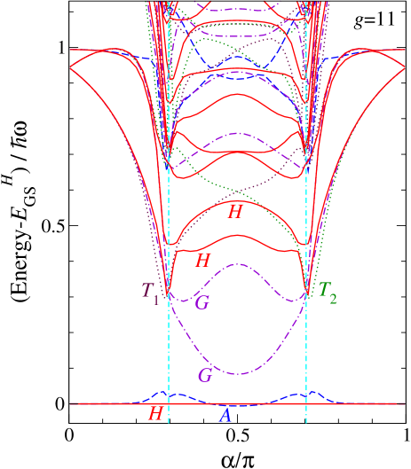
Figure 12: Low-energy region of the vibronic spectrum of a single $H$ mode coupled to a $h$ level, as a function of $\alpha$, for $g=11$. Energies are referred to the lowest $H$ state.

Figure 12 reports the excitation energies of several low-lying vibronic states for $g=11$ (intermediate/strong coupling). The tunneling partners are visible at the low-energy end, with the crossing to an $A$ GS in the range $0.42\pi\lesssim\alpha\lesssim 0.58\pi$. The coupling is not strong enough to have the higher vibronic levels organized according to the harmonic frequencies of Fig. 3 throughout the $\alpha$ range, but similar trends are already recognizable: in particular for $\alpha\lesssim 0.2\pi$ and $\alpha\gtrsim 0.8\pi$, the vibronic levels follow quite closely the harmonic frequencies of Fig. 3, and their overtones and combinations. As observed in the discussion of Fig. 8, the vibronic spectrum in the strong tunneling regions at and around the flat-trough values $\alpha=\alpha_{s}$ and $\pi-\alpha_{s}$ is extremely congested: only the lowest-lying states are drawn in figure. Accordingly, most vibronic levels undergo a fast movement in that region, but always evolve continuously across $\alpha=\alpha_{s}$ and $\pi-\alpha_{s}$. In the limit of infinitely large $g$, the singular behavior of Fig. 3 would eventually emerge even in the exact quantum spectrum. The very large slope in the $\alpha$ dependence of many vibronic energies may prove useful in future precise determinations of the JT coupling parameters from spectroscopic data.

IV Photoemission spectra

Several spectral properties of experimental interest are readily accessed by the exact diagonalization method at hand. Photoemission spectra (PES) involving the quintet $h$ molecular orbital are of course affected by JT coupling to the degenerate vibrations. If, as is usually the case, the photoemitted electron kinetic energy is much larger than $\hbar\omega$, photoemission occurs in a time much shorter than that characteristic of phonon dynamics. In this limit, it is convenient to apply the sudden approximation Cederbaum77 ; Koppel84 , where the photoemission process is described simply by the operator $\hat{c}_{m\sigma}$ suddenly destroying a spin-$\sigma$ electron in orbital component $m$ of the quintet level. The phonon shakeup contributions to the PES are obtained in terms of the matrix elements of this hole-creation operator $\hat{c}_{m\sigma}$ between the initial configuration and the final vibronic states. If we assume that the initial temperature is negligible ($k_{\rm B}T\ll\hbar\omega$, only the GS $|{\rm GS}\rangle$ is initially populated), then the PES intensity for the creation of a spin-$\sigma$ hole in orbital $m$ is

$$I_{m\sigma}(E)\propto\sum_{f}\left|\langle f|\hat{c}_{m\sigma}|{\rm GS}\rangle\right|^{2}\,\delta\!\left(E-E_{f}\right)\,,$$ (7)

where averaging over the components is implied whenever $|{\rm GS}\rangle$ is degenerate. If the individual contributions of different orbital and spin component are not separate, the total PES intensity is then

$$I(E)=\frac{1}{10}\sum_{m\sigma}I_{m\sigma}(E)\,.$$ (8)

For generic occupancy of the $h$ level, the spectrum is generally affected not only by JT, but also by intra-shell electron-electron repulsion, and the ensuing multiplet structure Qiu01 ; Lueders02 ; Lueders03 : calculation of the PES in such conditions must take into account several other system-specific interactions. It thus goes beyond the study of the single-mode rather general model considered in this work. However, electron-electron repulsion plays no role in two relevant cases, which are therefore completely described by the JT Hamiltonian $\hat{H}$ of Eqs. (1)-(4): (i) when a single electron occupies the quintet orbital in the initial state, and (ii) when the orbital quintet is initially completely full and photoemission produces a single hole in the final state. In the first case, JT only affects the initial configuration, while in the second case, JT only affects the final states. The application of exact diagonalization to the two cases separately provides spectra where all non-adiabatic effects and phenomena neglected in the Frank-Condon approximation Mahapatra99 are fully included.

IV.1 JT in the initial states

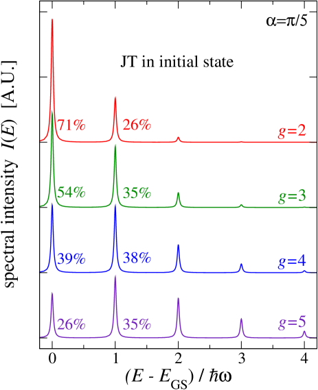
Figure 13: Zero-temperature PES obtained by fast removal of the single electron from a $h$ orbital coupled to a single $H$ mode, for several values of the coupling $g$, and $\alpha=\pi/5$. Energies are referred to the GS; a phenomenological broadening HWHM=$0.02\,\hbar\omega$ provides a finite width to the peaks. Fractional spectral weights of the 0-phonon and 1-phonon line are listed.

When JT only affects the initial states, the molecule is instantaneously brought from the multi-well intrinsically nonadiabatic vibronic GS to a linear superposition of the final harmonic oscillator states. According to Eqs. (7) and (8), the peaks in the spectrum are located at the final-state energies $E_{f}$, which here simply involve single or multiple excitations of the harmonic phonon $\hbar\omega$. The spectrum is therefore a sequence of regularly spaced peaks, with intensity of the 0, 1, 2… -phonon line proportional to the square modulus of the corresponding total component in the initial vibronic GS.

Figure 13 presents precisely a spectrum with this simple structure, for an $H$ mode characterized by $\alpha=\pi/5$. According to the standard electron-phonon (non-JT) Frank-Condon picture, the percentage of spectral intensity displaced away from the 0-phonon to the multi-phonon excitations increases with the distance between the initial and final equilibrium configurations, which, in turn, is proportional to the linear coupling parameter $g$.

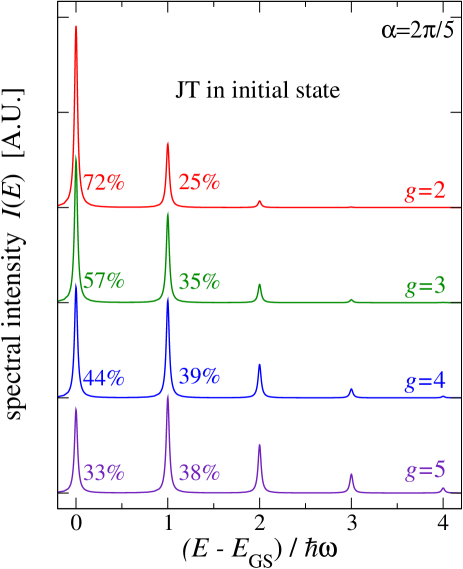
Figure 14: Same as Fig. 13 for $\alpha=2\pi/5$.

The situation is qualitatively similar for $\alpha=2\pi/5$ (and for the case of a $G$ mode, which is omitted for brevity). The only quantitative difference to observe in Fig. 14 compared to Fig. 13 is that for $\alpha=2\pi/5$ spectral weight is preferentially transfered to the 1-phonon line, while for $\alpha=\pi/5$ it is more equally distributed among several phonon excitations.

The spectra in Figs. 13-14 are obtained by means of a complete Lanczos calculation of the GS wavefunction. This is straightforward, as long as zero temperature is addressed as in the present work. If instead finite-temperature was to be considered, many initial vibronic states would be required for a thermal average, and this is generally a difficult task for the Lanczos method Bordoni04 : completely different techniques, e.g. based on Monte Carlo, could prove more convenient there.

IV.2 JT in the final states

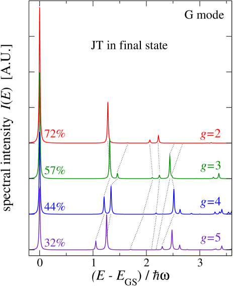
Figure 15: Zero-temperature PES obtained by fast removal of an electron from a filled $h$ orbital coupled to a single $G$ mode, for several values of the coupling $g$. Energies are referred to the GS; a phenomenological broadening HWHM=$0.01\,\hbar\omega$ provides a finite width to the peaks. Fractional spectral weights of the “zero-phonon” line are listed.

When JT affects the final states, the energies $E_{f}$ marking the PES peaks are the vibronic energies of Figs. 2, 4-12. The transparent structure of a harmonic spectrum is now lost. However, the calculation of the PES is straightforward, as $|{\rm GS}\rangle$ is now the 0-phonon state of the filled-shell non-JT molecule . The symmetry of the state $\hat{c}_{m\sigma}|{\rm GS}\rangle$ occurring in the matrix element of Eq. (7) is that of the electronic operator $\hat{c}_{m\sigma}$, namely $H$. As a consequence, only transitions to $H$ final states $\langle f|$ are possible, while matrix elements to all other vibronic states vanish by symmetry. Peaks occur therefore only at the energies marked by the solid lines in Figs. 2, 4-12.

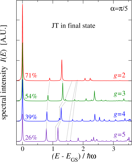
Figure 16: Zero-temperature PES obtained by fast removal of an electron from a filled $h$ orbital coupled to a single $H$ mode, for several values of the coupling $g$ and, $\alpha=\pi/5$. Energies are referred to the GS; a phenomenological broadening HWHM=$0.01\,\hbar\omega$ provides a finite width to the peaks. Fractional spectral weights of the “zero-phonon” line are listed.

Figure 15 reports the computed PES for a coupled $G$ mode and a few intermediate values of $g$. The positions of the low-lying peaks correspond to the solid lines of Fig. 2b, and are readily followed. Strong intensity transfers due to level crossings are well visible. The intensity of the “zero-phonon” line (better referred to as the vibronic GS) decreases steadily as $g$ increases : the intensity lost there redistributes across an intricate vibronic spectrum.

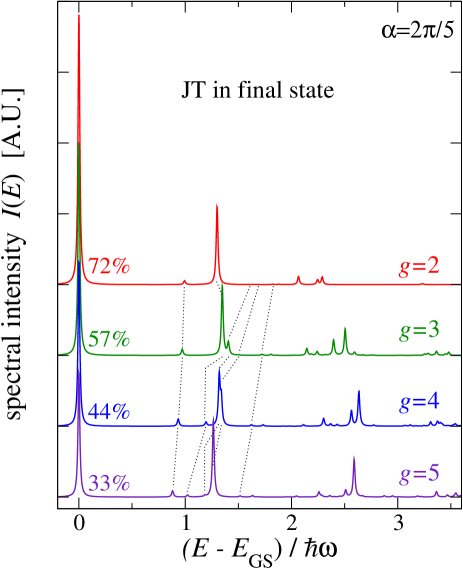
Figure 17: Same as Fig. 16 for $\alpha=2\pi/5$.

Figures 16 and 17 report the computed PES for a coupled $H$ mode characterized by the same value of $\alpha$ of Fig. 6 ($\pi/5$, producing $D_{5}$ minima) and of Fig. 9 ($2\pi/5$, producing $D_{3}$ minima) respectively. The positions and intensities of several low-lying peaks can be traced: several intensity transfers due to level crossings are well visible. Again, the intensity of the “zero-phonon” line decreases consistently as $g$ is increased, while the intensity lost there redistributes across a rather dense spectrum of vibronic levels.

Figures  15-17 illustrate in detail the general finding Manini03 that in the PES of dynamic JT system with weak to intermediate coupling, the “1-phonon line” splits into essentially two features, usually with most spectral weight in the upper peak, blue-shifted up to 30% higher energy than $\hbar\omega$. The blue shift of the 1-phonon satellite is not specific to the $h\otimes(G+H)$ JT model. For example, similar conclusions apply to the $e\otimes E$ problem Bersuker . Indeed a 15% blue shift of the first vibronic satellite is clearly observable in the PE spectra of benzene Baltzer97etal .

A general feature of the displayed PES is that the perturbative structure of $n$-phonon states, still fairly well recognizable for $g=2$), is rapidly lost in the PES for $g\gtrsim 3$. The only other general consideration we can draw from these spectra is that not much regularity is to be expected: unless coupling is very weak, phonon shakeups in the PES from a JT molecule build very intricate spectral structures, which are strongly $g$-dependent (also $\alpha$-dependent, for $H$ modes), even for a single phonon mode.

V Discussion

Understanding the general features of a vibronic spectrum is a necessary step towards the interpretation and assignment of the spectra of molecules and molecular ions. This has been undertaken and carried out quite extensively for electronic doublets, triplets Bersuker ; Englman ; Martinelli91etGrosso and more complex electronic configurations Qiu01 ; Sookhun03 ; Li03 . The present paper fills a gap in the theory of icosahedral systems, providing general guidelines for the interpretation of vibronic PES of the electronic quintet in the $h\otimes(G+H)$, restricting to the idealization of a single mode. In practical applications, the situation is much more intricate. All actual icosahedral systems are many-mode systems, where the inter-mode interaction generates a much less coherent spectrum than simple non-JT phonons Gattari03 . The present theory allows the basic understanding of the PES of icosahedral systems wherever the coupling to a single high-energy mode is dominant, the other couplings only contributing to the background. The couplings of fullerene C₆₀ are approximately of this kind, and the spectral of Sect. IV.2 allow to rationalize some observed PES features in terms of an effective single-mode theory.

On the other hand, the spectra of Sect. IV.1 describe a situation where a single electron in a $h$ state is rapidly removed. This cannot occur in practically accessible ionic states of C₆₀, but could well occur in singly charged negative ions of higher icosahedral fullerenes, under the condition that the LUMO is a quintet. By particle-hole symmetry, the same theory applies to inverse PES, where a single hole in a quintet is filled. This is relevant, e.g. for inverse PES of C${}_{60}^{+}$.

The difficulty of the many-modes JT Bersuker ; ManyModes is that no linear superposition of the spectra of single modes occurs (except for the weak-coupling limit). This means that any quantitative description of the dynamics requires to include all modes together in a single calculation. The method of Lanczos exact diagonalization used in the present work is by no means limited to the single-mode case. Indeed, Ref. Manini03, deals successfully with the intricacies of the C₆₀ many-mode problem, also accounting for thermal effects. The same theory used in Sect. IV.2 for PES could be applied to an optical transition from a nondegenerate electronic $a$ state to a final $h$ state, if that dipole-forbidden transition could be realized. Modifications of the same method could be employed to study phonon shakeups in optical absorption/emission in dipole allowed transitions involving electronic degenerate states at both sides: these are often associated to “product” JT systems Qiu01 ; Ceulemans00 , and with due account of “term” exchange interactions, JT would account for the vibronic “decorations” of the spectra, not unlike PES. More applications of the Lanczos method (including generalizations thereof Meyer89 ) to other spectroscopical applications are therefore expected in the future.

Appendix A Exact eigenenergies

	1	2	5	10	15
$A$	3.724144	3.163979	0.990680	-3.888699	-10.881188
$A$	5.094787	4.788557	2.428383	-2.782559	-9.799588
$T_{1/2}$	2.903273	2.634575	1.098218	-3.511597	-10.336507
$T_{1/2}$	3.745236	3.221392	1.222379	-3.110401	-9.893907
$G$	2.799066	2.355251	0.503564	-3.987637	-10.885576
$G$	3.859923	3.502678	1.672126	-3.351358	-10.317040
$H$	1.882022	1.581814	0.105229	-4.046978	-10.887960
$H$	2.819443	2.411645	0.673159	-3.612510	-10.340670
$H$	2.992497	2.859999	1.158021	-3.449058	-10.317965
$H$	3.746243	3.228490	1.359820	-3.191928	-9.925392
$H$	3.793559	3.345318	1.504876	-3.113374	-9.815484
$H$	3.888832	3.646643	1.810633	-2.941030	-9.781893

Table 1: Exact eigenenergies of several low-lying vibronic states of $h\otimes G$ linear JT for selected values of the coupling parameter $g$. Energies are in units of $\hbar\omega$.

$g$	1	2	5	10	15
$A$	3.269039	2.704296	0.014206	-7.605244	-20.103759
$A$	4.416117	4.031416	1.213521	-6.611668	-19.106543
$T_{1/2}$	3.349001	2.940441	0.696237	-6.663875	-19.157685
$G$	3.349001	2.940441	0.696237	-6.663875	-19.157685
$G$	3.405264	3.109744	0.907404	-6.663079	-19.157685
$H$	2.376848	2.025472	-0.135556	-7.605387	-20.103759
$H$	3.405223	3.107032	0.786076	-6.663301	-19.157685
$H$	3.405264	3.109744	0.907404	-6.663079	-19.157685
$H$	4.245489	3.651009	1.018708	-6.613430	-19.106543

Table 2: Exact eigenenergies of several low-lying vibronic states of $h\otimes H$ linear JT for $\alpha=0$ and selected values of the coupling intensity $g$. Energies are in units of $\hbar\omega$.

$g$	1	2	5	10	15
$A$	3.286920	2.838680	1.066520	-3.082956	-9.369654
$A$	4.309107	3.872518	2.044770	-2.121879	-8.473972
$T_{1}$	3.318833	2.915855	1.247562	-2.696110	-8.854724
$T_{1}$	4.287826	3.838287	2.068227	-1.958552	-8.086429
$T_{2}$	3.434328	3.237084	1.880242	-2.280608	-8.537845
$T_{2}$	4.285742	3.829377	2.016910	-2.178646	-8.345314
$G$	3.333101	2.956614	1.370430	-2.614428	-8.851809
$G$	3.364209	3.029490	1.485305	-2.346950	-8.538216
$H$	2.382792	2.089510	0.694933	-3.124845	-9.370196
$H$	3.345469	2.978750	1.375559	-2.572543	-8.849910
$H$	3.510110	3.423708	1.778880	-2.340165	-8.537793
$H$	4.242742	3.729200	1.947019	-2.305749	-8.491719

Table 3: Same as Table 2, for $\alpha=\pi/4$.

$g$	1	2	5	10	15
$A$	3.282422	2.807794	0.866002	-3.650697	-10.518971
$A$	4.431838	4.165069	2.165531	-2.669479	-9.635062
$T_{1/2}$	3.390187	3.098692	1.498544	-3.029840	-9.956428
$G$	3.305993	2.869310	1.027386	-3.525390	-10.511108
$G$	3.321806	2.908694	1.077499	-3.306272	-9.969104
$H$	2.381251	2.074260	0.534055	-3.662262	-10.516120
$H$	3.406622	3.132388	1.463674	-3.184920	-9.966811
$H$	3.478854	3.325880	1.517402	-3.071858	-9.959172
$H$	4.227504	3.672462	1.693740	-2.935829	-9.678823
$H$	4.252143	3.734125	1.787623	-2.900136	-9.660194

Table 4: Same as Table 2, for $\alpha=\pi/2$.

Tables 1-4 collect a number of exact vibronic eigenenergies of the orbital-quintet single-mode linear JT model. Note that $E_{\rm clas}$ was not subtracted here, therefore the tabulated energies represent precisely the eigenvalues of the Hamiltonian as defined in Eq. (1). All reported digits are significant. Extra degeneracies are apparent in all tables except Table 3 ($\alpha=\pi/4$). However, the apparent degeneracy between the $A$ states and $H$ states for $g=15$, $\alpha=0$ (Table 2) only indicates that the (tunneling) splitting between these states is smaller than the energy resolution of the diagonalization (see also Fig. 4).

References

- (1) M. Lüders, N. Manini, P. Gattari, and E. Tosatti, Eur. Phys. J. B 35, 57 (2003).
- (2) D. K. Bohme, Can. J. Chem. 77, 1453 (1999).
- (3) A. Ceulemans, J. Chem. Phys. 87, 5374 (1987).
- (4) A. Ceulemans, and P. W. Fowler, J. Chem. Phys. 93, 1221 (1990).
- (5) M. Szopa and A. Ceulemans, J. Phys. A 30, 1295 (1997).
- (6) C. P. Moate, M. C. M. O’Brien, J. L. Dunn, C. A. Bates, Y. M. Liu, and V. Z. Polinger, Phys. Rev. Lett. 77, 4362 (1996).
- (7) C. P. Moate, J. L. Dunn, C. A. Bates, and Y. M. Liu, J. Phys.: Condens. Matter 9, 6049 (1997).
- (8) V. Z. Polinger, Adv. Quantum Chem. 44, 59 (2003).
- (9) P. De Los Rios, N. Manini, and E. Tosatti, Phys. Rev. B 54, 7157 (1996).
- (10) N. Manini and P. De Los Rios, Phys. Rev. B 62, 29 (2000).
- (11) N. Manini, P. Gattari, and E. Tosatti, Phys. Rev. Lett. 91, 196402 (2003).
- (12) N. Manini and E. Tosatti, Phys. Rev. B 58, 782 (1998).
- (13) P. De Los Rios and N. Manini, in Recent Advances in the Chemistry and Physics of Fullerenes and Related Materials: Volume 5, edited by K. M. Kadish and R. S. Ruoff (The Electrochemical Society, Pennington, NJ, 1997), p. 468.
- (14) A. Auerbach, N. Manini, and E. Tosatti, Phys. Rev. B 49, 12998 (1994).
- (15) H. Koizumi and I. B. Bersuker, Phys. Rev. Lett. 83, 3009 (1999).
- (16) E. Lijnen and A Ceulemans, Adv. Quantum Chem. 44, 183 (2003).
- (17) A. Abragam and B. Bleaney, Electron Paramagnetic Resonance of Transition Ions (Oxford University Press, London, 1970).
- (18) P. Brühwiler, A. J. Maxwell, P. Balzer, S. Andersson, D. Arvanitis, L. Karlsson, and N. Mårtensson, Chem. Phys. Lett. 279, 85 (1997).
- (19) S. E. Canton, A. J. Yencha, E. Kukk, J. D. Bozek, M. C. A. Lopes, G. Snell, and N. Berrah, Phys. Rev. Lett. 89, 045502 (2002).
- (20) N. Manini and E. Tosatti, Phys. Rev. Lett. 90, 249601 (2003).
- (21) J. L. Dunn, C. A. Bates, C. P. Moate, and Y. M. Liu, J. Phys.: Condens. Matter 15, 5697 (2003).
- (22) N. Manini, A. Dal Corso, M. Fabrizio, and E. Tosatti, Philos. Mag. B 81, 793 (2001).
- (23) M. Lüders, A. Bordoni, N. Manini, A. Dal Corso, M. Fabrizio, and E. Tosatti, Philos. Mag. B 82, 1611 (2002).
- (24) P. H. Butler, Point Group Symmetry Applications (Plenum, New York, 1981).
- (25) U. Öpik and M. H. L. Pryce, Proc. Roy. Soc. A 238, 425 (1957).
- (26) N. Manini and P. De Los Rios, J. Phys.: Condens. Matter 10, 8485 (1998).
- (27) E. Lo and B. R. Judd, Phys. Rev. Lett. 82, 3224 (1999).
- (28) B. R. Judd, in The Dynamical Jahn-Teller Effect in Localized Systems, edited by Y. E. Perlin and M. Wagner (Elsevier, Amsterdam 1984), p. 87.
- (29) J. Jaklic and P. Prelovsek, Adv. Phys. 49, 1 (2000).
- (30) H.-D. Meyer and S. Pal, J. Chem. Phys. 91, 6195 (1989).
- (31) M. Lueders and N. Manini, Adv. Quantum Chem. 44, 289 (2003).
- (32) C. A. Bates, J. L. Dunn, and E. Sigmund, J. Phys. C: Solid State Phys. 20, 1965 (1987).
- (33) L. S. Cederbaum, W. Domcke, H. Köppel, and W Vonniessen, Chem. Phys. 26, 169 (1977).
- (34) H. Köppel, W. Domcke, and L. S. Cederbaum, Adv. Chem. Phys. 57, 59 (1984).
- (35) Q. C. Qiu, L. F. Chibotaru, and A. Ceulemans, Phys. Rev. B 65, 035104 (2001).
- (36) S. Mahapatra, L. S. Cederbaum, and H. Köppel, J. Chem. Phys. 111, 10452 (1977).
- (37) A. Bordoni and N. Manini - cond-mat/0407132, in print in Fullerenes. Recent Advances in the Chemistry and Physics of Fullerenes and Related Materials - Volume 14, ed. by P. V. Kamat, F. DSouza, D. M. Guldi, and S. Fukuzumi (The Electrochemical Society, Pennington, NJ).
- (38) I. B. Bersuker and V. Z. Polinger, Vibronic Interactions in Molecules and Crystals (Springer-Verlag, Berlin, 1989).
- (39) P. Baltzer et al., Chem. Phys. 224, 95 (1997).
- (40) R. Englman, The Jahn Teller Effect in Molecules and Crystals (Wiley, London, 1972).
- (41) L. Martinelli et al., Phys. Rev. B 43, 8395 (1991); G. Grosso and G. Pastori Parravicini, Solid State Physics (Academic Press, San Diego, 2000), Ch. XII.7.
- (42) S. S. Sookhun, C. A. Bates, J. L. Dunn, and W. Diery, Adv. Quantum Chem. 44, 319 (2003).
- (43) H. Li, V. Z. Polinger, J. L. Dunn, and C. A. Bates, Adv. Quantum Chem. 44, 89 (2003).
- (44) P. Gattari, Diploma thesis, http://www.mi.infm.it/manini/theses/gattari.pdf .
- (45) A. Ceulemans and Q. C. Qiu, Phys. Rev. B 61, 10628 (2000).