Influence of magnetic fields on cold collisions of polar molecules

Abstract

We consider cold collisions of OH molecules in the ${}^{2}\Pi_{3/2}$ grounds state, under the influnce of a magnetic field. We find that modest fields of several thousand gauss can act to suppress inelastic collisions of weak-field seeking states by two orders of magnitude. We attribute this suppression to two factors: (i) An indirect coupling of the entrance and the exit channel, in contrast to the effect of an applied electric field; and (ii) the realtive motion of the entrance and exit scattering thresholds. In view of these results, magnetic trapping of OH may prove feasible.

I Introduction

As the experimental reality of trapping ultra-cold polar molecules approaches, a clear understanding is needed of how the molecules interact in the trap environment. On the most straightforward level, collisions are essential for cooling the gas by either evaporative or sympathetic cooling methods. A high rate of elastic collisions is desirable, while a low rate of exothermic, state-changing collisions is essential if the cold gas is to survive at all. Furthermore, a clear understanding of 2-body interactions allows one to construct a realistic model of the many body physics in this dilute system bec_rev .

One promising strategy for trapping ultracold molecules might be to follow up on successes in trapping of cold atoms, and to construct electrostatic Bethlem ; Meerakker or magneto static Weinstein traps that can hold molecules in a weak-field-seeking state. Cold collisions of polar molecules in this environment have been analyzed in the past, finding that inelastic collision rates were unacceptably high in the presence of the electric field, limiting the possibilities for stable trapping AA_PRA . Ref. AA_PRA found that the large inelastic rates were due to the strong dipole-dipole interaction coupling between the molecules. One important feature of the dipole-dipole interaction is its comparatively long range. Even without knowing the details of the short-ranged molecule-molecule interactions, the dipole forces alone were sufficient to change the internal molecular states. Indeed, a significant finding was that for weak-field seekers, the molecules are prevented from approaching close to one another due to a set of long-range avoided crossings. Therefore, a reasonably accurate description of molecular scattering may be made using the dipolar forces alone AA_PRL .

A complimentary set of theoretical analyses have considered the problem of collisional stability of paramagnetic molecules in a magnetostatic trap. For example, the weak-field-seeking states of molecules are expected to survive collisions with He buffer gas atoms quite well BohnPRA2000 ; Krems1 . Collisions of molecules with each other are also expected to preserve their spin orientation fairly well, and hence remain trapped AAPRA2001 . However, this effect is mitigated in the presence of a magnetic field Volpi ; Krems2 .

So far, no one appears to have considered the influence of magnetic fields on cold molecule-molecule collisions where both species have electric dipole moments. In this paper we approach this subject, by considering cold OH(${}^{2}\Pi_{3/2}$)-OH(${}^{2}\Pi_{3/2}$) collisions in a magnetic field. To the extent that the applied electric field is zero, one might expect that dipole forces average to zero and thus do not contribute to de-stabilizing the spin orientation. It turns out that this is not quite correct, and that dipole-dipole forces still dominate long-range scattering. However, applying a suitably strong magnetic field turns out to mitigate this effect significantly. Interestingly, even in this case the residual second-order dipole interactions are sufficiently strong to restrict scattering to large intermolecular separation

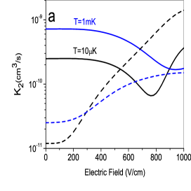
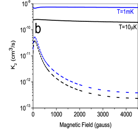
Figure 1: Thermally averaged rate constants for collisions of weak-field seeking sates of OH, as a fucntion of applied electric field (a) and magnetic field (b). In both cases, solid lines denote elastic scattering rates, while dashesd lines denote inelastic scattering rates. Two temperatures are considered. Applying an electric fields drives the inelastic collisions rates up while applied magnetic field drives inelastic collision rates down.

The main result of the paper is summarized in Figure 1, which contrasts the influence of electric and magnetic fields. Figure 1(a) plots the elastic (solid curves) and inelastic (dashed curves) collision rate constants for OH molecules in their $|FM_{F}\epsilon\rangle=|22-\rangle$, weak-field-seeking hyperfine state (for details on quantum numbes, see below). As the electric field is increased, the elastic rate constant grows to alarmingly large values, making the gas collisionally unstable, as was shown in Ref. AA_PRA . Figure 1(b), which is new to this paper, shows the analogous rate constants in a magnetic field (in both cases the field is assumed to lie along the positive z axis of the laboratory reference frame). In this case the magnetic field has the effect of suppressing collisions, all the way down to a rate constant of $2\times 10^{-13}$ cm³/sec at fields of $B=3000$ gauss. These results are moreover fairly robust against raising the temperature to the merely cold (not ultracold) temperatures, $\sim 1mK$, attainable in buffer-gas loading or Stark slowing experiments. This is good news for experiments – it implies that cooling strategies that rely on collisions may be feasible, provided a suitably large bias magnetic field is applied.

Our main goal here is to analyze the suppression of rates in a magnetic field. The organization is as follows. First we review the relevant molecular structure, and especially the Stark and Zeeman effects, to illustrate their complementary natures. We then present an overview of the scattering model, including a review of the dipole-dipole interaction. Finally we present an analysis of the system in a magnetic field using a reduced channel model that encapsulates the essential collision physics. Finally the model is qualitatively understood using the adiabatic representation.

II Electric versus magnetic fields applied to molecules

Both the Stark and Zeeman effects in molecules have a similar form, since both arise as the scalar product of a dipole moment with an external field. Their influence on the molecule is quite different, however, since they act on fundamentally different degrees of freedom. The electric field is concerned primarily with where the charges are in the molecule, whereas the magnetic field is concerned with where they are going. This is of paramount importance, since it implies that the electric field is a true vector (odd under the parity operation), whereas the magnetic field is a pseudovector (even under parity) Jackson . An electric field will therefore mix parity states of a molecule, while a magnetic field will mix states only of a given parity. This distinction is explored further in Ref. Freed ; here we will only focus on those aspects of immediate relevance to our project.

The rest of this paper will, fundamentally, restate this fact in the context of scattering, and follow up the consequences that arise from it. To set the context of this discussion, and to fix our notation, we first consider the molecules in the absence of external fields.

II.1 Molecular structure in zero external field

The OH radical has a complicated ground state structure which includes rotation, parity, nuclear spin, electronic spin and orbital degrees of freedom. We assume that the vibrational degrees of freedom are frozen out at low temperatures, hence treat the molecules as rigid rotors. We further assume that perturbations due to far away rotational levels are weak. We do, however, include perturbatively the influence of the $\Omega=1/2$ fine structure level, as described in Ref. AA_PRA .

The electronic ground state of OH is ${}^{2}\Pi$, with $\Omega=3/2$ . OH is an almost pure Hund’s case (a) molecule, meaning the electronic degrees of freedom are strongly coupled to the intermolecular axis. The electronic state of the molecule in the $J$ basis is denoted by $|JM_{J}\Omega\rangle|\Lambda\Sigma\rangle$ where $J$ is the total electronic angular momentum, $M_{J}$ is its projection onto the lab axis and $\Omega$ is $J$’s projection onto the molecular axis. $\Sigma$ and $\Lambda$ are the projection of the electron’s spin and orbital angular momentum onto the molecular axis, and their sum equals $\Omega$ ($=\Sigma+\Lambda$). The electronic degrees of freedom, $|\Lambda\Sigma\rangle$, will be suppressed for notational simplicity because they are constant for all the collisional processes we consider.

To describe the molecular wave function we assume a rigid rotor, $\langle\alpha,\beta,\gamma|JM_{J}\Omega\rangle=\sqrt{2J+1\over 8\pi^{2}}D^{J\star}_{M_{J}\Omega}(\alpha,\beta,\gamma)$, where$(\alpha,\beta,\gamma)$ are the Euler angles defining the molecular axis and $D^{J\star}_{M_{J}\Omega}$ is a Wigner D-function. It is necessary for a $\Pi$ state molecule to use the parity basis because OH has a $\Lambda$-doublet splitting which separates the two parity states ($e/f$). The $\Lambda$-doublet arises from a coupling to a near by $\Sigma$ state. It is the coupling of the $\Sigma$ state to $\Pi$ state of the same parity which breaks the degeneracy of the two $\Pi$ parity states Brown .

In the parity basis the molecular wave function is written

$$|JM_{J}\bar{\Omega}\pm\rangle=\left({|JM_{J}\Omega\rangle+\epsilon|JM_{J}-\Omega\rangle\over\sqrt{2}}\right).$$ (1)

Where $\epsilon=+(-)$ represents the $e$ ($f$) state, and $\bar{\Omega}=|\Omega|$. It should be noted that the sign of $\epsilon$ is not the parity, rather parity is equal to $\epsilon(-1)^{(J-1/2)}$ Brown . Thus for the ground state of OH where $J=3/2$, parity is equal to $-\epsilon$. Throughout the paper we use $\pm$ denote the sign of $\epsilon$, not parity. In the parity basis there is no dipole moment, because this basis is a linear combination of electric dipole “up” and “down”. This fact has important implications for the dipole-dipole interaction.

Including the hyperfine structure is important because the most dominant loss processes are those that change the hyperfine quantum number of one or both of the scattering molecules. The hyperfine structure arises from interaction of the electronic spin with the nuclear spin ($I$) which must then be included in the molecular basis set. In the hyperfine basis the OH states are $|FM_{F}\pm\rangle$, where ${\bf F}={\bf J+I}$ and $M_{F}$ is its projection onto the lab axis. Here we suppress $\bar{\Omega}$ in the notation, as its value is understood. To construct basis functions with quantum number $F$ we expand in Clebsh-Gordon coefficients:

$$|FM_{F}\pm\rangle=\sum_{M_{J}M_{I}}|JM_{J}\bar{\Omega}\pm\rangle|IM_{I}\rangle\langle JM_{J}IM_{I}|FM_{F}\rangle.$$ (2)

Relevant molecular energy scales for the scattering problem are the $\Lambda$-doublet splitting which is $\Delta\sim 0.0797K$, the hyperfine splitting is $\Delta_{hf}\sim 0.0038K$. OH also has an electric dipole moment is $\mu\sim 1.668D$. Throughout this paper we use Kelvin $(K)$ as the Energy unit, except in the instances of thermally averaged observables. For reference, $0.64K=1cm^{-1}$.

II.2 Stark Effect in OH

As noted above, the distinguishing feature of the Stark effect is that it mixes molecular states of opposite parity separated by the $\Lambda$ doublet splitting. A consequence of this is that the Stark energies vary quadratically with electric field at low fields, and linearly only at higher fields. The field where this transition occurs is given roughly by equating the field’s effect ${\vec{\mu}_{E}}\cdot{\vec{E}}$ to the $\Lambda$ doublet splitting (here ${\vec{\mu}_{E}}$ is the molecule’s electric dipole moment, and ${\vec{E}}$ is the field. In OH, this field is approximately $\emph{E}_{0}\sim\Delta/2\mu_{\emph{E}}\sim 1000(V/cm)$.)

The Stark Hamiltonian has the form

$$H_{S}=-{\vec{\mu}_{{\emph{E}}}}\cdot{\emph{\bf}E}$$ (3)

where we take the field to be in the $\hat{z}$ direction. In the basis in which $\Omega$ has a definite sign, the matrix elements are well known Townes :

$$\langle JM_{J}\Omega|H_{S}|JM_{J}\Omega\rangle={-\mu_{\emph{E}}\emph{E}\Omega M_{J}\over J(J+1)}.$$ (4)

In the Stark effect there is a degeneracy between states with the same sign of $\Omega M_{J}$, meaning $\pm M_{J}$ are degenerate in an electric field. We can recast the Stark Hamiltonian into the $J$-parity basis set from Eqn. (1). Doing so, we find

$$\langle JM_{J}\bar{\Omega}\epsilon|H_{S}|JM_{J}\bar{\Omega}\epsilon^{\prime}\rangle={-\mu_{\emph{E}}\emph{E}\bar{\Omega}M_{J}\over J(J+1)}\left({1-\epsilon\epsilon^{\prime}\over 2}\right).$$ (5)

In this expression, the factor $(1-\epsilon\epsilon^{\prime})/2$ explicitly represents the electric field coupling between states of opposite parity, since it vanishes for $\epsilon=\epsilon^{\prime}$.

Finally, using the definition of the $F$-parity basis in Eqn. (2), we arrive at the working matrix elements of the Stark effect:

$$\langle FM_{F}\epsilon|H_{S}|F^{\prime}M_{F}\epsilon^{\prime}\rangle=-{\mu_{\emph{E}}\emph{E}}\left({1+\epsilon\epsilon^{\prime}(-1)^{J+J^{\prime}+2\bar{\Omega}+1}\over 2}\right)$$

$$\times(-1)^{J+J^{\prime}+F+F^{\prime}+I-M_{F}-\bar{\Omega}+1}[F,F^{\prime},J,J^{\prime}]$$

$$\times\left(\begin{array}[]{ccc}J&1&J^{\prime}\\ -\bar{\Omega}&0&\bar{\Omega}^{\prime}\end{array}\right)\left(\begin{array}[]{ccc}F^{\prime}&1&F\\ M_{F}&0&-M_{F}\end{array}\right)\left\{\begin{array}[]{ccc}F&F^{\prime}&1\\ J^{\prime}&J&I\end{array}\right\}.$$ (12)

In this notation $[j_{1},j_{2},...]=\sqrt{(2j_{1}+1)(2j_{2}+1)(...)}$. Figure 2 shows the energy levels of OH in the presence of an electric field. Both parity states are shown, labeled $e$ and $f$. An essential point of Fig. 2 is that the $e$ and $f$ states repel as the electric field in increased. This means the all of the $f$ ($e$) states increase (decrease) in energy as the field in increased, implying that states of the same parity stay close together in energy as the field is increased. This fact has a crucial effect on the inelastic scattering as we will show.

The highest-energy state in Fig. 2 is the stretched state with quantum numbers $|FM_{F}\epsilon\rangle=$ $|22-\rangle$. It is this state whose cold collisions we are most interested in, because i) it is weak-field seeking, and ii) its collisions at low temperature result almost entirely from long-range dipole-dipole interactions AA_PRA . Molecules in this state will suffer inelastic collisions to all of the other internal states shown. The rate constant shown in Figure 1 is the sum of all rate constants for all such processes.

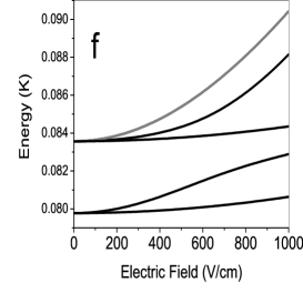
Figure 2: Stark effect for the ground state of OH with the hyperfine structure accounted for. In zero field the f states and the e states are separated by the $\Lambda$-doublet energy. The Gray line indicates the state of interest for our analysis, the $|22-\rangle$ state. An important feature of this interaction is that the opposite parity states repel and thus like parity state stay close together in energy.

II.3 Zeeman Effect in OH

When OH is in an external magnetic field the electron’s orbital motion and intrinsic magnetic dipole moment both interact with the field. The interaction is described by the Zeeman Hamiltonian which is

$$H_{Z}=-{\bf\mu}_{B}\cdot{\bf B}=\mu_{0}({\bf L}+g_{e}{\bf S})\cdot{\bf B}.$$ (13)

Here $\mu_{0}$ is the Bohr magneton and $g_{e}$ is the electron’s g factor ($g_{e}\sim 2.002$). As above, we assume the field to be in the laboratory $\hat{z}$ direction. In the $J$ basis, the Zeeman Hamiltonian takes the form herzberg

$$\langle JM_{J}\Omega|H_{Z}|JM_{J}\Omega\rangle={\mu_{0}B(\Lambda+g_{e}\Sigma)\Omega M_{J}\over J(J+1)}.$$ (14)

This is quite similar to the equivalent expression (4) for the Stark effect, except that the electron’s $g$-factor plays a role. Interestingly, for a ${}^{2}\Pi$ state the prefactor $(\Lambda+g_{e}\Sigma)\Omega$ is always greater than zero. We now recast the Zeeman interaction into the $J$-parity basis set (1). This gives us

$$\langle JM_{J}\bar{\Omega}\epsilon|H_{Z}|JM_{J}\bar{\Omega}\epsilon^{\prime}\rangle={\mu_{0}B\left(\bar{\Lambda}+g_{e}\bar{\Sigma}\right)\bar{\Omega}M_{J}\over J(J+1)}\delta_{\epsilon\epsilon^{\prime}}$$ (15)

for $\bar{\Omega}=3/2$ states, and

$$\langle JM_{J}\bar{\Omega}\epsilon|H_{Z}|JM_{J}\bar{\Omega}\epsilon^{\prime}\rangle={\mu_{0}B\left(\bar{\Lambda}-g_{e}\bar{\Sigma}\right)\bar{\Omega}M_{J}\over J(J+1)}\delta_{\epsilon\epsilon^{\prime}}$$ (16)

for $\bar{\Omega}=1/2$ states. Notice that for $\bar{\Omega}=1/2$, the orbital and spin contributions to the molecular magnetic moment nearly cancel, to within the deviation of $g_{e}/2$ from one. For the $\bar{\Omega}=3/2$ states of interest to us, however, the magnetic moment remains large.

The key feature of the Zeeman matrix element (15) is that it is diagonal in $\epsilon$, in contrast to the Stark matrix element. This trait persists in the hyperfine basis as well, where the matrix elements are

$$\langle FM_{F}\epsilon|H_{Z}|F^{\prime}M_{F}\epsilon^{\prime}\rangle=$$

$${\mu_{0}B(\bar{\Lambda}+g_{e}\bar{\Sigma})}\left({1+\epsilon\epsilon^{\prime}(-1)^{(J+J^{\prime}+2\bar{\Omega})}\over 2}\right)$$

$$\times(-1)^{J+J^{\prime}+F+F^{\prime}+I-M_{F}-\bar{\Omega}+1}[F,F^{\prime},J,J^{\prime}]$$ (17)

$$\times\left(\begin{array}[]{ccc}J&1&J^{\prime}\\ -\bar{\Omega}&0&\bar{\Omega}^{\prime}\end{array}\right)\left(\begin{array}[]{ccc}F^{\prime}&1&F\\ M_{F}&0&-M_{F}\end{array}\right)\left\{\begin{array}[]{ccc}F&F^{\prime}&1\\ J^{\prime}&J&I\end{array}\right\}.$$ (24)

Figure 3 shows the Zeeman energies in the hyperfine basis, for low (Fig. 3(a)) and high (Fig. 3(b)) fields. For OH in the ${}^{2}\Pi_{3/2}$ state, the parity factor $\left({1+\epsilon\epsilon^{\prime}(-1)^{(J+J^{\prime}+2\bar{\Omega})}\over 2}\right)$ reduces simply to $\delta_{\epsilon\epsilon^{\prime}}$. Because the magnetic field respects parity, figure 3 (b) amounts to two copies of the same energy level diagram, separated in energy by the lambda doublet energy. For small magnetic fields the molecular $g$-factor is $g_{mag}^{OH}\propto(F^{2}+J^{2}-I^{2})$, and is always positive for OH. This is in contrast to the low field magnetic moment of alkali atoms which is $g_{mag}^{alkali}\propto(F^{2}-J^{2}-I^{2})$ (and where $J$, of course, refers to the sum of orbital and spin angular momenta). In Eqn. (24) for $\bar{\Omega}=1/2$ the factor $\bar{\Lambda}+g_{e}\bar{\Sigma}$ goes to $\bar{\Lambda}-g_{e}\bar{\Sigma}$.

,

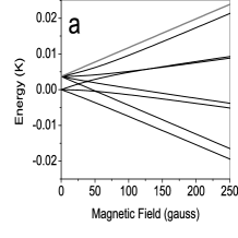
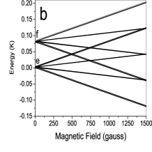
Figure 3: Zeeman effect for the ground state of OH, in low (a) and high (b) fields. This plot is the same for both the $e$ and $f$ states for zero electric field because the Zeeman interaction respects preserves parity. The $|22-\rangle$ state is indicated in gray.

III Scattering Hamiltonian

A complete potential energy surface for the interaction of two OH molecules, including the relatively long-range part most relevant to cold collisions, is at present unavailable. Certain aspects of this surface have, however, been discussed surface . For the time being, we will follow our previous approach of focusing exclusively on the dipole-dipole interaction. It appears that molecules in the highest weak-field-seeking states are mostly insensitive to short-range effects.

The “raw” scattering channels have the form $|F_{1}M_{F_{1}}\epsilon_{1}\rangle|F_{2}M_{F_{2}}\epsilon_{2}\rangle|lm_{l}\rangle$, which specifies the internal state of each molecule and the partial wave $l$ describing the relative orbital angular momentum of the molecules. In a field, of course, the hyperfine and parity quantum numbers are no longer good. It is therefore essential to consider a set of scattering channels “dressed” by the appropriate field. This is achieved by diagonalizing the Stark or Zeeman Hamiltonian of each molecule, including the $\Lambda$ doubling and hyperfine structure. The resulting eigenvectors then comprise the molecular basis used to construct the scattering Hamiltonian. Field dressing is essential because otherwise non-physical couplings between channels presist to infinite separation. The diagonal contributions of the Stark and Zeeman Hamiltonian in the field dressed basis define to the scattering thresholds as $R\rightarrow\infty$.

The channels involved in a given scattering process are further constrained by symmetries. Namely, scattering of identical bosons restricts the basis set to even values of $l$ only. In addition, the cylindrical symmetry enforced by the external field guarantees that the total projection of angular momentum on the field axis, $M=M_{F_{1}}+M_{F_{2}}+m_{l}$, is a conserved quantity.

The scattering wave function is expanded in these field-dressed channels, leading to a set of coupled-channel Schrödinger equations

$$\left({-\hbar^{2}\over 2m_{r}}{d^{2}\over dR^{2}}\underline{1}+{\hbar^{2}\hat{l}^{2}\over 2m_{r}R^{2}}\underline{1}+\underline{V}({\bf R})+\underline{H}_{FS}\right)\vec{\psi}(R)=E\vec{\psi}(R),$$ (25)

where $\vec{\psi}$ is the multichannel wavefunction and $m_{r}$ is the reduced mass. The operators $\underline{H}_{FS}$ denotes the fine strucutre, including the effect of an electric or magnetic field. (In this paper we do not yet include the simultaneous effect of both fields.)

In Eqn. (25), the operator $\underline{V}$ represents the interaction between the molecules. We are most interested in the dominate dipole-dipole interaction whose general operator form is

$$H_{\mu\mu}=-\ {3(\hat{\bf R}\cdot\hat{\bf\mu}_{1})(\hat{\bf R}\cdot\hat{\bf\mu}_{2})-\hat{\bf\mu}_{1}\cdot\hat{\bf\mu}_{2}\over R^{3}}.$$ (26)

where ${\bf\hat{\mu}}_{i}$ the electric dipole of molecule $i$, $R$ is the intermolecular separation, and ${\bf\hat{R}}$ is the unit vector defining the intermolecular axis. This interaction is conveniently re-written in terms of tensorial operators as follows Brink :

$$H_{\mu\mu}=-{\sqrt{6}\over R^{3}}\sum_{q}(-1)^{q}C^{2}_{q}\cdot(\mu_{1}\otimes\mu_{2})^{2}_{-q}.$$ (27)

Here $C^{2}_{q}(\theta,\phi)$ is a reduced spherical harmonic that acts only on the relative angular coordinate of the molecules, while $(\mu_{1}\otimes\mu_{2})^{2}_{-q}$ is the second rank tensor formed from two rank-1 operators, $\mu_{i}$ that act on the state of the $i^{th}$ molecule. These first rank operators are written as reduced spherical harmonics, $C_{q}^{1}(\alpha\beta)$ where $\alpha$ and $\beta$ are two of the Euler angles of the rigid rotator wavefunction. With this form of the dipole-dipole interaction, we can then evaluate the matrix element.

In the hyperfine parity basis (2) the matrix elements are AA_PRA

$$\langle 12lm_{l}|H_{\mu\mu}|1^{\prime}2^{\prime}l^{\prime}m_{l}^{\prime}\rangle= {\sqrt{6}\mu^{2}_{{\emph{E}}}\over R^{3}}[l,l^{\prime},J_{1},J^{\prime}_{1},J_{2},J^{\prime}_{2},F_{1},F^{\prime}_{1},F_{2},F^{\prime}_{2}]\left({1+\epsilon_{1}\epsilon^{\prime}_{1}(-)^{J_{1}+J_{1}^{\prime}+2\bar{\Omega}_{1}+1}\over 2}\right)\left({1+\epsilon_{2}\epsilon^{\prime}_{2}(-)^{J_{2}+J_{2}^{\prime}+2\bar{\Omega}_{2}+1}\over 2}\right)$$

$$\times (-1)^{(1+F_{1}+F_{1}^{\prime}+F_{2}+F_{2}^{\prime}+J_{1}+J_{1}^{\prime}+J_{2}+J_{2}^{\prime}+M_{1}+M_{2}-\Omega_{1}^{\prime}-\Omega_{2}^{\prime}+M_{l})}$$

$$\times \left(\begin{array}[]{ccc}1&1&2\\ M_{F_{1}}-M_{F_{1}^{\prime}}&M_{F_{2}}-M_{F_{2}^{\prime}}&M_{l}-M_{l}^{\prime}\end{array}\right)\left(\begin{array}[]{ccc}J_{1}&1&J_{1}^{\prime}\\ -\bar{\Omega}_{1}&0&\bar{\Omega}_{1}\end{array}\right)\left(\begin{array}[]{ccc}J_{2}&1&J_{2}^{\prime}\\ -\bar{\Omega}_{2}&0&\bar{\Omega}_{2}\end{array}\right)$$ (34)

$$\times \left(\begin{array}[]{ccc}1&F_{1}&F_{1}^{\prime}\\ M_{F_{1}}-M_{F_{1}^{\prime}}&-M_{F_{1}}&M_{F_{1}^{\prime}}\end{array}\right)\left(\begin{array}[]{ccc}1&F_{2}&F_{2}^{\prime}\\ M_{F_{2}}-M_{F_{2}^{\prime}}&-M_{F_{2}}&M_{F_{2}^{\prime}}\end{array}\right)$$ (39)

$$\times \left(\begin{array}[]{ccc}l^{\prime}&2&l\\ M_{l^{\prime}}&M_{l}-M_{l^{\prime}}&-M_{l}\end{array}\right)\left(\begin{array}[]{ccc}l^{\prime}&2&l\\ 0&0&0\end{array}\right)\left\{\begin{array}[]{ccc}F_{1}&F_{1}^{\prime}&1\\ J_{1}^{\prime}&J_{1}&I\end{array}\right\}\left\{\begin{array}[]{ccc}F_{2}&F_{2}^{\prime}&1\\ J_{2}^{\prime}&J_{2}&I\end{array}\right\}.$$ (48)

A central feature of this matrix element is the factor $\left(1-\epsilon_{1}\epsilon^{\prime}_{1}\right)\left(1-\epsilon_{2}\epsilon^{\prime}_{2}\right)$, using $J_{i}=J_{i}^{\prime}=\bar{\Omega}_{i}=3/2$. As a consequence of this factor, matrix elements diagonal in parity identically vanish in zero electric field. Instead, for example, two $f$-parity states only interact with one another via coupling to a channel consisting of two $e$-parity states.

This dependence on parity is perhaps not unexpected, since the dipole-dipole force is of course transmitted by the dipole moment of the first molecule producing an electric field that acts on the second molecule. But in a state of good parity, the first molecule does not have a dipole moment until it is acted upon by the second molecule. Thus, both molecules must simultaneously mix states of opposite parity to interact. Notice that in the presence of an electric field, the dipoles are already partially polarized, and this restriction need not apply; the scattering channels are already directly coupled. This change is of decisive importance in elucidating the influence of electric fields on collisions. In a magnetic field, by contrast, parity remains conserved and the interactions are intrinsically weaker as a result.

IV Inelastic Rates of OH-OH collisions in external fields

We move now to the consequences of the interaction (48) on scattering. Scattering calculations are done using the log-derivative propagator method johnson . To ensure convergence at all collision energies and applied fields, it was necessary to include partial waves up to $l=6$, and to carry the propagation out to an intermolecular distance of $R=10^{4}(a.u.)$ before matching to long-range wave functions. Cross sections and rate constants are computed in the standard way for anisotropic potentials Bohn00PRA .

We remind the reader that throughout we consider collisions of molecules initially in their $|FM_{F}\epsilon\rangle=$ $|22-\rangle$ states, which are weak-field seeking for both electric and magnetic fields. Thus for a scattering process incident on an s- partial wave, the incident channel will be written $|i\rangle=|F_{1}M_{F_{1}}\epsilon_{1}\rangle|F_{2}M_{F_{2}}\epsilon_{2}\rangle|lm_{l}\rangle=$ $|22,-\rangle|22,-\rangle|00\rangle$.

In the following, we will make frequent reference to “energy gap suppression” of collision rates. This notion arises from a perturbative view of inelastic collisions, in which case the transition probability amplitude is proportional to the overlap integral

$$\int dR\psi_{i}(R)V_{if}(R)\psi_{f}(R)$$ (49)

where $\psi_{i,f}$ denote the incident and final channel radial wave functions, and ${V}_{if}$ is the coupling matrix element between them. In our case, $\psi_{i}$ will have a long de Broglie wavelength corresponding to its essentially zero collision energy. The de Broglie wavelength of $\psi_{f}$ will instead grow smaller as the energy gap $E_{i}-E_{f}$ between incident and final thresholds grows. Thus the integral in (49), and correspondingly the collision rates, will diminish. For this reason, the collisions we consider tend to favor changing the hyperfine states of the molecules over changing the parity states, since the hyperfine splitting of OH is smaller than the $\Lambda$-doubling.

IV.1 Electric Field Case

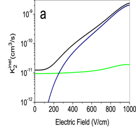
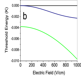
Figure 4: (a) Total (black) and selected partial (color) inelastic rates for OH-OH collisions as a function of electric field. The green curve is the dominant zero field inelastic loss process to channel $|10-\rangle|22-\rangle$ (green). In the presence of the field, a different channel, $|21-\rangle|22-\rangle$, becomes dominant (blue). (b) The thresholds for these exit channels, relative to the incident threshold.

To calculate scattering in the presence of an electric field, we only need to include partial waves $l=0,2$ for numerical accuracy of $K^{inel}_{2}$ for the field range that we consider, $E\leq 1000(V/cm)$, and at a collision energy of $10^{-5}$ K. Here we are only interested in the trend and identification of the loss mechanism. To numerically converge the inelastic rates at higher field values, where the induced dipoles are large, naturally requires more partial waves.

Figure 4 (a) shows the total (black) and partial (color) inelastic rate constant $K_{2}^{inel}$ as a function of the electric field (compare Fig. 1 (a)). Even in zero field, where the dipolar forces nominally average out, the rate constant is large, comparable to the elastic rate constant. This fact attests to the strength of dipolar forces in OH, even in second order.

The green line in Fig. 4(a) represents losses to the dominant zero field loss channel $|10-\rangle|22-\rangle|22\rangle$. The blue curve in Fig. 4 (a) represents instead the dominant loss process at higher electric field values, in channel $|21-\rangle|22-\rangle|21\rangle$. Whereas the former rate remains relatively insensitive to field, the latter rises dramatically.

This behavior arises from two competing tendencies in an electric field. The first is the increasing mixing of different parity states as the field is turned on, leading to an increasing strength of the direct dipole-dipole coupling that affects both exit channels. This additional coupling would, in general, cause inelastic rates to rise. It is, however, offset by the competing tendency for inelastic rates to become less likely when the change in relative kinetic energy of the collision partners is larger. Fig. 4(b) shows the threshold energies for the two exit channels in Fig. 4(a), versus field, with zero representing the energy of the incident threshold. Here it is evident that loss to the channel $|22-\rangle|10-\rangle|22\rangle$ (green line) is accompanied by a large gain in kinetic energy, whereas loss to channel $|21-\rangle|22-\rangle|21\rangle$ (blue line) gains comparatively little kinetic energy, and thus the later channel more strongly affected by the increased coupling generated by the field.

IV.2 Magnetic Field Case

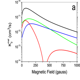
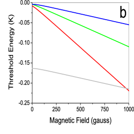
Figure 5: (a) The total (black) and partial (color) inelastic rates for OH-OH collisions as a function of magnetic field. The colors are explained in the text. (b) The corresponding thresholds, referred to the incident channel’s threshold ($E_{i}=0$). The lowest curve is one possible intermediate channel.

To gain insight into the suppression of the inelastic rates in a magnetic field (Fig. 5 (a)), calculations were at a representative collision energy $E=10^{-5}K$. To converge the calculations in high field (B$\geq 1500$ gauss) required partial waves $l=0,2,4,6$. We have only considered collisions with incident partial wave $l=0$, since higher partial wave contributions, while they exist, only contribute to rates at the fraction of a precent level.

Because the electric field remains zero, parity is still a rigorously good quantum number. Therefore states of the same parity are not directly coupled. Nevertheless, the dominant loss channels in a magnetic field share the parity of the incident channel wave function, $|i\rangle=|22,-\rangle|22,-\rangle|00\rangle$. Figure 5 (a) illustrates this by showing the total (black) and partial (color) inelastic rates as a function of the magnetic field. The loss rates shown correspond to the exit channels $|f\rangle=$ $|10-\rangle|22-\rangle|22\rangle$(green), $|11-\rangle|22-\rangle|41\rangle$(blue), and $|10-\rangle|10-\rangle|44\rangle$(red).

Since direct coupling to these final channels is forbidden to the dipolar interaction, all coupling must occur through some intermediate channel $|int\rangle$. Moreover, owing to the parity selection rules in the matrix element (48), this intermediate channel must have parity quantum numbers $\epsilon_{1}=\epsilon_{2}=+$. Since this coupling is second order, the dominant exit channels can consist of both d-wave ($l_{f}=2$) and g-wave ($l_{f}=4$) contributions, in contrast to the electric field case.

The primary feature of the inelastic rates in Fig. 5 (a) is that they decrease significantly at large field. This decline is the main reason for optimism regarding evaporative cooling strategies in OH; an applied bias field of 3000 Gauss can reduce the inelastic rate constant to below $2\times 10^{-13}$ cm³/sec, see Figure 1. The cause of this decrease can be traced directly to the relative separation of the incident and final channel thresholds, along with the indirect nature of the coupling.

To see this, we reduce the model to its essential ingredients: (1) a strong dipole-dipole interaction, (2) the relative motion of the thresholds as the magnetic field is tuned, (3) an extremely exothermic intermediate channel and (4) the centrifugal barrier in the final and intermediate channels. The Hamiltonian for a reduced model is $H_{Model}=T_{0}+V_{Model}$, where $T_{0}$ is the kinetic energy operator and $V_{Model}$ in matrix form is

$$V_{Model}=\left(\begin{array}[]{ccc}E_{i}&0&a/R^{3}\\ 0&E_{f}+c_{f}/R^{2}&b/R^{3}\\ a/R^{3}&b/R^{3}&E_{int}+c_{int}/R^{2}\\ \end{array}\right).$$ (53)

Here $c_{j}$ is a centrifugal repulsion $c_{j}=\hbar^{2}l_{j}(l_{j}+1)/2m_{r}$, $a$ and $b$ are dipole-dipole coupling strengths, and $E_{j}$ are the threshold energies for the $j^{th}$ channel. The channels $\{i,f,int\}$ have quantum numbers $(\epsilon_{1}\epsilon_{2})^{i}=(\epsilon_{1}\epsilon_{2})^{f}=(--)$ and $(\epsilon_{1}\epsilon_{2})^{int}=(++)$. The incident channel has partial wave $l_{i}=0$, while dipole coupling selection rules allow $l_{int}=2$, and $l_{f}=2$ or $l_{f}=4$.

The model Hamiltonian (53) explicitly excludes direct coupling between incident and final channels, whereas coupling is mediated through the $int$ channel. Parameters characteristic of the physical problem are $a=0.12$ (a.u.), $b=0.10$ (a.u.), $E_{i}=0$, $E_{f}=-0.003\rightarrow-0.1(K)$, and $E_{int}=-0.17(K)$, $l_{i}=0$, $l_{f}=2$ or $l_{f}=4$ and $l_{int}=2$. Because of the energy gap separation losses to the intermediate channels are negligible. We find, in addition, that moving $E_{int}$ has little effect on the rate constants for loss to channel $f$.

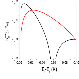
Figure 6: Inelastic rate constants for the 3-channel model system, Eq. 53, as function of initial and final threshold separation. The two curves are for $d$ and $g$-wave exit channels black and red, respectively. In $g$-wave channel $K_{2}^{inel}$ evolves more slowly as the thresholds are separated.

Fig. 6 shows the inelastic rates computed within this model. This three channel model does a reasonable job of mimicking the prominent features of the full calculation, including the eventual and lasting decrease in rates as the states are separated in energy. In addition, the g-wave rates decay more slowly as a function of field than do the d-wave rates, consistent with the full calculation (compare Fig. 5). The declining values of the rate constant cannot, however, be attributed to a simple overlap integral of the form (49), since the incident and final channels are not directly coupled. We therefore present a more refined adiabatic analysis of this process in the next subsection.

IV.3 Adiabatic Analysis of the magnetic field case

To understand the system’s magnetic field behavior we analyze the reduced channel model (53) in the adiabatic representation AA_FL ; child . This representation assumes that $R$ is a “slow” coordinate. At every $R$ we diagonalize the Hamiltonian in all remaining degrees of freedom. Since it is not rigorously true that $R$ varies infinitely slowly, the residual nonadiabatic couplings can be accounted for in the kinetic energy operator. Written more formally we diagonalize

$$\underline{W}=\left({\hbar^{2}l(l+1)\over 2m_{r}R^{2}}\underline{1}+\underline{V}(R)+\underline{H}_{Z}\right)$$ (54)

where the terms are the centrifugal barrier, potential matrix including dipole-dipole interaction and the Zeeman Hamiltonian. Diagonalizing the matrix in Eq. 54, we get $\underline{W}|\alpha(R)\rangle=U_{\alpha}(R)|\alpha(R)\rangle$ where $U_{\alpha}(R)$ are the eigenvalues and $|\alpha(R)\rangle$ are the eigenvectors. With the eigenvectors we are able to form a linear transformation $\underline{X(R)}$ which transforms between the diabatic and adiabatic representations, ie $\underline{X^{T}}\underline{W}(R)\underline{X}=\underline{U}(R)$. The eigenvalues and eigenvectors have radial dependence, but for notational simplicity $(R)$ will be suppressed hereafter.

To distinguish between adiabatic and diabatic representations we use Greek letters ($\alpha,\beta,...$) to denote the adiabatic channels and Roman letters (i,j,…) to denote diabatic channels. When considering specific inelastic processes in the diabatic basis we denote initial and final channels as $i$ and $f$ and for the adiabatic channels as $\iota$ and $\varphi$. In the limit $R\rightarrow\infty$, the two sets of channels coincide.

Figure 7: The relevant adiabatic potential curves for the OH-OH system. Shown are two different values of the final threshold energy $E_{i}-E_{f}=5mK$ (a) and $E_{i}-E_{f}=15mK$ (b)

A partial set of adiabatic potential curves generated in this way is shown in Fig. 7, exhibiting an avoided crossing at $R=150$. Thus molecules incident on the uppermost channel scatter primarily at large values of $R$. This point has been made in the past when an electric field is applied AA_PRA ; here we note that it is still true in zero electric field, and that scattering calculations can proceed without reference to short-range dynamics.

The transformation between the representations is $R$ dependent implying that the channel couplings shift from the potential to the kinetic energy operator. Using the adiabatic representation changes Eq. 25 to

$$\left(\underline{X}^{T}{-\hbar^{2}\over 2m_{r}}{d^{2}\over dR^{2}}\underline{X}+\underline{U}\right)\vec{\xi}(R)=$$

$$\left({-\hbar^{2}\over 2m_{r}}\left({d^{2}\over dR^{2}}+2\underline{P}{d\over dR}+\underline{Q}\right)+\underline{U}\right)\vec{\xi}(R)=E\vec{\xi}(R).$$ (55)

Here $\vec{\xi}=\underline{X}^{T}\vec{\psi}$.

To get the channel couplings in the adiabatic picture we need matrix elements of the derivative operators, defined as $P_{\alpha\beta}=\langle\alpha|{d\over dR}|\beta\rangle$. We evaluate the the $P_{\alpha\beta}$ matrix, the dominant off-diagonal channel coupling, using the Hellmann-Feynman theorem child

$$P_{\alpha\beta}={\sum_{kl}X_{\alpha k}^{T}\nabla V_{kl}X_{l\beta}\over U_{\alpha}-U_{\beta}}.$$ (56)

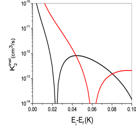
Figure 8: Inelastic rate constants as estimated by the adiabatic distorted wave Born approximation for the 3-channel system. The black curve is for a d-wave exit channel and the red for a g-wave exit channel.

Scattering amplitudes are then easily estimated in the adiabatic distorted-wave Born approximation (ADWBA). Namely, we construct incident and final radial wave functions $\phi_{\iota,\varphi}$ that propagate according to the adiabatic potentials $U_{\iota,\varphi}$. In terms of these adiabatic wavefunctions, the scattering $T$-matrix is given by an overlap integral analogous to Eqn. 49

$$T_{\iota\varphi}={\pi\hbar^{2}\over m_{r}}\langle\phi_{\iota}|{\overleftarrow{d/dR}\underline{P}+\underline{P}\overrightarrow{d/dR}\over\sqrt{2}}|\phi_{\varphi}\rangle.$$ (57)

Here $\overleftarrow{d/dR}$ ($\overrightarrow{d/dR}$) is the radial derivative operator acting to the left (right). The cross section for identical bosons is $\sigma_{\iota\varphi}={8\pi\over k_{\iota}^{2}}|T_{\iota\varphi}|^{2}$. From here we are able to numerically calculate a rate constant for inelastic loss $K_{2}^{inel}=v_{\iota}\sigma_{\iota\varphi}$ where $v_{\iota}$ is the asymptotic velocity given by $\sqrt{2U_{\iota}(R\rightarrow\infty)/m_{r}}$.

The result of the ADWBA is shown in figure 8. The two curves are for $d$ (black) and $g$-wave (red) inelastic channels. Several key features are present that also occur in the full calculation, namely: (1) the inelastic rate goes down with increasing threshold separation. (2) there is a zero in the rates as seen in Fig. 5 (3) the $g$-wave inelastic rate goes more slowly than the $d$-wave as seen in the model and the full calculation. The ADWBA accounts for all of these. The first feature, diminishing rates, still arises from an energy gap suppression, since the de Broglie wavelengths of incident and final channel still do not match well. In the ADWBA this process is further helped along by the fact that the residual channel coupling, represented by $P$, is localized near the avoided crossings of the adiabatic potential curves.

The ADWBA helps to visualize this suppression, as shown by the sample wave functions in Fig. 9. This figure shows $\psi_{\iota}$, ${d\over dR}\psi_{\varphi}$, and $P_{\iota\varphi}$ for various values of $E_{f}$. Varying $E_{f}$ mimics the threshold motion of the system. The values of $E_{f}$ of Figure 9 are (a) $E_{f}=-6mK$, (b) $E_{f}=-22mK$, and (c) $E_{f}=-62mK$. The effect of the different $E_{f}$s leave $\psi_{\iota}$ mostly unchanged, however $\psi_{\varphi}$ becomes more exothermic and therefore more oscillatory ($\lambda_{db}$ clearly shortens). Moreover, the dominant coupling region, where $P_{\iota\varphi}$ peaks, moves to shorter $R$ as $E_{f}$ increases. This motion is obvious from the avoided crossing in Fig. 7.

The transition amplitude in the ADWBA is proportional to the integral of the product of the three quantities in Fig. 9. Because of the shortening of the de Broglie wavelength in the exit channel, this integral will eventually vanish, accounting for the zero in the inelastic rates. The total rate will, in general, not vanish, since there are many exit channels, and they will experience the destructive interference at different values of the threshold, hence at different fields.

Finally, the $g$-wave inelastic rates are not so strongly affected by the separation of $E_{i}$ and $E_{f}$ because the g-wave centrifugal barrier is larger, meaning a greater energy is required to change the wave function at short range such that velocity node can pass through the coupling region. The zero in this rate constant will thus occur at larger threshold separations.

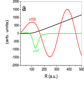
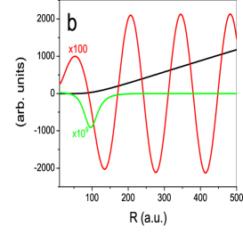
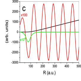
Figure 9: Illustrations of the origin of the zero in the partial rates. Each panel shows curves $\psi_{\iota}$, ${d\over dR}\psi_{\varphi}\times 100$ and $P_{\iota\varphi}$ $\times 10^{9}$. The plots are for different final energies and inelastic rate from the Born approximation are (a) $E_{f}=-6mK$ and $K^{inel}_{\iota\varphi}=5\times 10^{-11}$ (b) $E_{f}=-22mK$ , $K^{inel}_{\iota\varphi}=5\times 10^{-14}$ (c) $E_{f}=-62mK$, $K^{inel}_{\iota\varphi}=6\times 10^{-13}$, see text for details.

V Conclusions

We have explored the influence of a magnetic field on the cold collision dynamics of polar molecules. The dipole-dipole interactions remain significant even in the absence of an electric field that polarizes the molecules. In general this implies that molecular orientations are unstable in collisions, making magnetic trapping infeasible. We have found, however, that a suitably strong magnetic field can mitigate this instability.

Beyond this result, we note that laboratory strength fields can exert comparable influence on cold collisions, if applied separately. A useful rule of thumb in this regard is that an electric field of 300 $V/cm$ acting on a 1 $Db$ dipole moment caues roughly the same energy shift as a 100 $gauss$ field acting on a 1 Bohr magneton magnetic moment. This raises the interesting question of how the two fields can be applied simultaneously, to exert even finer control over collision dynamics. This will be the subject of future investigations.

- (1) For a reivew see M.A. Baranov, et. al, Physica Scripta, T102, 764 (2002).
- (2) H.L. Bethlem, G. Berden, F.M.H. Crompvoets, R.T. Jongma, A.J.A. van Roij, and G. Meijer, Nature 406, 491 (2000).
- (3) S.Y.T. Meerakker, et. al, physics/0407116 (2004).
- (4) Weinstein et. al, Nature 395, 148 (1998)
- (5) A.V. Avdeenkov and J.L. Bohn, Phys. Rev. A 66, 052718 (2002).
- (6) A.V. Avdeenkov and J.L. Bohn, Phys. Rev. Lett. 90, 043006 (2003).
- (7) J. L. Bohn, Phys. Rev. A 62, 032701 (2000).
- (8) R. V. Krems,A. Dalgarno, N. Balakrishnan, and G. C. Groenenboom, Phys. Rev. A, 67 060703(R) (2003).
- (9) A. V. Avdeenkov and J. L. Bohn, Phys. Rev. A 64, 052703 (2001).
- (10) A. Volpi and J.L. Bohn, Phys. Rev. A 65, 052712 (2002).
- (11) R. V. Krems, J. Chem. Phys., 120 2296 (2004); R. V. Krems, H.R. Sadeghpour, A. Dalgarno, D. Zgid, J. Klos, and G. Chalasinski, Phys Rev. A, 68 051401(R) (2004)..
- (12) J. D. Jackson, Classical Electrodynamics (2nd Edition, Wiley, New York, 1975, p. 249).
- (13) Karl Freed, J. Chem. Phys. 45, 4214 (1966).
- (14) J. Brown and A. Carrington, Rotational Spectroscopy of Diatomic Molecules, (Cambridge, Cambridge, 2003).
- (15) C. H. Townes and A. L. Schawlow Microwave Spectroscopy, (Dover, New York, 1975)
- (16) G. Herzberg Molecular Spectra and Molecular Structure: vol. 1 Spectra of Diatomic molecules. (Kreiger, Florida, 1950).
- (17) B. Kuhn, et. al J. Chem. Phys. 111, 2565 (1999); L. B. Harding J. Phys. Chem. 95, 8653 (1991); R. Chen, G. Ma and H. Guo, J. Chem. Phys. 114, 4763 (2000).
- (18) D. M. Brink and G. R. Satchler, Angular Momentum, (Clardeon Press, Oxford, 1993).
- (19) B. R. Johnson, J. Comput. Phys. 13, 445 (1973).
- (20) J. L. Bohn, Phys. Rev. A 62, 032701 (2000).
- (21) A. V. Avdeenkov, D. C. E. Bortolotti, and J. L. Bohn, PRA 6912710 (2004).
- (22) M. S. Child, Molecular Collision Theory, (Dover, New York, 1974).