“Dressing” lines and vertices in calculations of matrix elements with the coupled-cluster method and determination of Cs atomic properties

Abstract

We consider evaluation of matrix elements with the coupled-cluster method. Such calculations formally involve infinite number of terms and we devise a method of partial summation (dressing) of the resulting series. Our formalism is built upon an expansion of the product $C^{\dagger}C$ of cluster amplitudes $C$ into a sum of $n$-body insertions. We consider two types of insertions: particle/hole line insertion and two-particle/two-hole random-phase-approximation-like insertion. We demonstrate how to “dress” these insertions and formulate iterative equations. We illustrate the dressing equations in the case when the cluster operator is truncated at single and double excitations. Using univalent systems as an example, we upgrade coupled-cluster diagrams for matrix elements with the dressed insertions and highlight a relation to pertinent fourth-order diagrams. We illustrate our formalism with relativistic calculations of hyperfine constant $A(6s)$ and $6s_{1/2}-6p_{1/2}$ electric-dipole transition amplitude for Cs atom. Finally, we augment the truncated coupled-cluster calculations with otherwise omitted fourth-order diagrams. The resulting analysis for Cs is complete through the fourth-order of many-body perturbation theory and reveals an important role of triple and disconnected quadruple excitations.

I Introduction

Coupled-cluster (CC) method Coester and Kümmel (1960); Čìžek (1966) is a powerful and ubiquitous technique for solving quantum many-body problem. Let us briefly recapitulate general features of the CC method, so we can motivate our further discussion. At the heart of the CC method lies the exponential ansatz for the exact many-body wavefunction

$$|\Psi_{i}\rangle=\exp(T_{i})|0_{i}\rangle=(1+T_{i}+\frac{1}{2!}T_{i}^{2}+\cdots)|0_{i}\rangle\,.$$ (1)

Here $T_{i}=\sum_{k}T_{i}^{(k)}$ is the cluster operator involving amplitudes $T_{i}^{(k)}$ of $k$-fold particle-hole excitations from the reference Slater determinant $|0_{i}\rangle$. The parametrization (1) is derived from rigorous re-summation of many-body perturbation theory (MBPT) series. From solving the eigenvalue equation one determines the cluster amplitudes and the associated energies. While the ansatz  (1) contains an infinite number of terms due to expansion of the exponent, the resulting equations for cluster amplitudes $T_{i}^{(k)}$ contain a finite number of terms. This simplifying property is unfortunately lost when the resulting wavefunctions are used in calculations of matrix elements: upon expansion of exponents the number of terms becomes infinite. Indeed, consider matrix elements of an operator $Z$, e.g., transition amplitude between two states

$$\mathcal{M}_{ij}=\frac{Z_{ij}}{\sqrt{N_{i}N_{j}}}\,,$$ (2)

with normalization $N_{i}=\langle\Psi_{i}|\Psi_{i}\rangle$. It is clear that both the numerator and denominator have infinite numbers of terms, e.g.,

$$Z_{ij}=\langle\Psi_{i}|Z|\Psi_{j}\rangle=\sum_{\lambda=0}^{\infty}\sum_{\mu=0}^{\infty}\frac{1}{\lambda!\mu!}\langle 0_{i}|(T_{i}^{\dagger})^{\lambda}\,Z\,(T_{j})^{\mu}|0_{j}\rangle\,.$$ (3)

In this paper we address a question of partially summing the terms of the above expansion for matrix elements, so that the result subsumes an infinite number of terms.

More specifically we are interested in transitions between states of univalent atoms, such as alkali-metal atoms. There has been a number of relativistic coupled-cluster calculations for these systems Blundell et al. (1989, 1991); Safronova et al. (1998, 1999); Sahoo et al. (2003); Gopakumar et al. (2002); Eliav et al. (1994). In particular, calculations Blundell et al. (1989, 1991); Safronova et al. (1998, 1999) ignore the non-linear terms ($\lambda>1$ and $\mu>1$) in the expansion (3); we will designate this approximation as linearized coupled-cluster (LCC) method. At the same time, it is well established that for the univalent atoms an important chain of many-body diagrams for matrix elements comes from so-called random-phase approximation (RPA). A direct comparison of the RPA series and the truncated LCC expansion in Ref. Derevianko and Emmons (2002) leads to a conclusion that a fraction of the RPA chain is missed due to the omitted non-linear terms. One of the methods to correct for the missing RPA diagrams has been investigated in Ref. Blundell et al. (1991). These authors replaced the bare matrix elements with the dressed matrix elements as prescribed by the RPA method. Such a direct RPA dressing involved a partial subset of diagrams already included in the CC method, i.e., it leads to a double-counting of diagrams. To partially rectify this shortcoming, the authors of Ref. Blundell et al. (1991) have manually removed certain leading-order diagrams, higher-order terms being doubly counted. Here we present an alternative infinite-summation scheme for RPA chain that avoids the double counting and thus a manual removal of the “extra” diagrams.

In addition to the RPA-like dressing of the coupled-cluster diagrams for matrix elements, we consider another subset of diagrams that leads to a dressing of particle and hole lines in the CC diagrams. The leading order corrections due to the dressing scheme presented here arise in the fourth order of MBPT, and in this paper we present a detailed comparison with the relevant fourth-order diagrams. Finally, we illustrate our approach with relativistic computation of hyperfine-structure constants and dipole matrix elements for Cs atom. In addition to dressing corrections we incorporate certain classes of diagrams from the direct fourth-order MBPT calculation (as in Ref. Derevianko and Emmons (2002); Cannon and Derevianko (2004)), so that the result is complete through the fourth order. To the best of our knowledge, the reported calculations are the first calculations for Cs complete through the fourth order of MBPT.

The paper is organized as follows. First, we present a more extensive discussion of the CC formalism in Section II. Further we dress particle and hole lines in Section IV, and discuss RPA-like dressing in Section V. The present paper may be considered as an all-order extension of forth-order calculation Derevianko and Emmons (2002); Cannon and Derevianko (2004), and in Section VI we present an illustrative comparison with the IV-order diagrams. Finally, the designed summation schemes are illustrated numerically in Section VII and the conclusions are drawn in Section VIII. Unless noted otherwise, atomic units, $\hbar=|e|=m_{e}\equiv 1$, are used throughout the paper. We follow the convention of Ref. Lindgren and Morrison (1986) for drawing Brueckner-Goldstone diagrams.

II Coupled-cluster formalism for univalent systems

In this Section we specialize our discussion of the coupled-cluster method to the atomic systems with one valence electron outside closed shell core. We review various approximations and summarize the CC formalism for calculation of matrix elements.

We are interested in solving the atomic many-body problem. The total Hamiltonian $H$ is partitioned as

$$H=H_{0}+G\,,$$ (4)

where $H_{0}$ is the suitably chosen lowest-order Hamiltonian and the residual interaction $G=H-H_{0}$ is treated as a perturbation. For systems with one valence electron outside closed-shell core, a convenient choice for $H_{0}$ is the frozen-core ($V^{N-1}$) Hartree-Fock Hamiltonian Kelly (1969). In the following, we explicitly specify the state $v$ of the valence electron, so that the proper reference eigenstate $|0_{i}\rangle$ of $H_{0}$ is $|0_{v}\rangle=a^{\dagger}_{v}|0_{c}\rangle$, where pseudo-vacuum state $|0_{c}\rangle$ specifies the occupied core.

For open-shell systems a general CC parametrization reads Lindgren and Morrison (1986)

$$|\Psi_{i}\rangle=\left\{\exp(T_{i})\right\}|\Phi_{i}\rangle\,,$$ (5)

where curly brackets denote normal product of operators. For univalent system the above ansatz may be simplified to

$$|\Psi_{v}\rangle=\exp\left(C\right)\,S_{v}a_{v}^{\dagger}|0_{c}\rangle=\left(\sum_{\mu=0}^{\infty}\frac{\left(C\right)^{\mu}}{\mu!}\right)\,S_{v}a_{v}^{\dagger}|0_{c}\rangle\,.$$ (6)

Here $C$ represents cluster operator involving (single, double, triple, etc.) excitations of core orbitals

$$C=C^{(1)}+C^{(2)}+\cdots=$$

$$\sum_{ma}\rho_{ma}~{}a_{m}^{\dagger}a_{a}+\frac{1}{2!}\sum_{mnab}\rho_{mnab}~{}a_{m}^{\dagger}a_{n}^{\dagger}a_{b}a_{a}+\cdots\,,$$

and $S_{v}$ incorporates additional excitations from the valence state $v$

$$S_{v}=1+S_{v}^{(1)}+S_{v}^{(2)}+\cdots$$

$$= 1+\sum_{m}\rho_{mv}~{}a_{m}^{\dagger}a_{v}+\sum_{mna}\rho_{mnav}~{}a_{m}^{\dagger}a_{n}^{\dagger}a_{v}a_{a}+\cdots\,.$$

In these formulae and throughout the paper we employ the following labeling convention: indexes $a,b,c,d$ denote single-particle states occupied in the core $|0_{c}\rangle$ and indexes $m,n,r,s,t$ stand for remaining (virtual/excited) orbitals. In this convention valence states $v$ and $w$ form a subset of the virtual orbitals. Finally, indexes $i,j,k,l$ stand for any of the above classes of single-electron orbitals. In Eqs. (II,II) the cluster amplitudes $\rho_{ij}$ stand for single-particle excitations and $\rho_{ijkl}$ for two-particle excitations, with an apparent generalization to $k$-fold excitation amplitudes.

Dictated by the computational complexity, in most applications the cluster operator is truncated at single and double excitations (CCSD approximation): $C\approx C^{(1)}+C^{(2)}$ and $S_{v}\approx 1+S_{v}^{(1)}+S_{v}^{(2)}$. A further linearized (LCCSD) approximation consists in neglecting non-linear terms in the expansion of exponent in Eq.(5), i.e.,

$$|\Psi_{v}\rangle^{\mathrm{LCCSD}}\equiv\left(1+S_{v}^{(1)}+S_{v}^{(2)}+C^{(1)}+C^{(2)}\right)|0_{v}\rangle\,.$$ (9)

As discussed in the introduction, the cluster amplitudes can be found from solving a proper analog of the eigen-value equation. We assume that these equations are solved and in a typical application we are faced with the necessity of computing matrix elements, Eq. (2), between two many-body wavefunctions $|\Psi_{v}\rangle$ and $|\Psi_{w}\rangle$. As demonstrated by Blundell et al. (1989), so-called disconnected diagrams Lindgren and Morrison (1986) in the numerator and the denominator of Eq. (2) cancel. Their final expression for the exact matrix element reads

$$\mathcal{M}_{wv} = \delta_{wv}\left(Z^{\mathrm{core}}\right)_{\mathrm{conn}}+$$ (10)

$$\frac{\left(Z_{wv}^{\mathrm{val}}\right)_{\mathrm{conn}}}{\left\{\left[1+\left(N_{v}^{\mathrm{val}}\right)_{\mathrm{conn}}\right]\left[1+\left(N_{w}^{\mathrm{val}}\right)_{\mathrm{conn}}\right]\right\}^{1/2}}\,,$$

where the matrix element $Z_{wv}$, Eq.(3), is split into core $Z^{\mathrm{core}}$ and valence $Z_{wv}^{\mathrm{val}}$ contributions, the diagrams comprising $Z^{\mathrm{core}}$ being independent of the valence indexes. The valence and core parts of the normalization factor $N_{v}$ are defined in a similar fashion. Notice that all the diagrams in Eq. (10) must be rigorously connected as emphasized by subscripts “$\mathrm{conn}$”. Since the total angular momentum of the closed-shell core is zero, the core contribution $Z^{\mathrm{core}}$ vanishes for non-scalar (and pseudo-scalar) operators and in the following discussion we will mainly focus on $Z_{wv}^{\mathrm{val}}$.

Blundell et al. (1989) have employed the LCCSD parametrization for the wavefunction (9) to derive 21 diagrams for $Z_{wv}^{\mathrm{val}}$ and 5 contributions to $N_{v}^{\mathrm{val}}$. The LCCSD contributions to $Z^{\mathrm{core}}$ can be found in Ref. Derevianko et al. (1998). It is the goal of this paper to go beyond these linearized LCCSD contributions. The LCCSD approximation will provide us with “skeleton” diagrams that will be “dressed” due to nonlinear CC terms. We display representative LCCSD diagrams in Fig. 1. In a typical calculation, the dominant correction to the Hartree-Fock (HF) value arise from RPA-type diagram (a) and Brueckner-orbital (BO) diagrams (c) and (d). (We retain the original enumeration scheme of Ref. Blundell et al. (1989) for the diagrams.) Here are the corresponding algebraic expressions for these LCCSD contributions

$$Z^{(\mathrm{HF})}_{wv} = z_{wv}\,,$$

$$Z^{(\mathrm{a})}_{wv} = \sum_{ma}z_{am}\tilde{\rho}_{wmva}+\mathrm{h.c.s.}\,,$$ (11)

$$Z^{(\mathrm{c})}_{wv} = \sum_{m}z_{wm}\rho_{mv}+\mathrm{h.c.s.}\,,$$

$$Z^{(\mathrm{d})}_{wv} = \sum_{mn}z_{mn}\rho^{\ast}_{mw}\rho_{nv}\,,$$

where $\mathrm{h.c.s.}$ denotes hermitian conjugation of preceding term with a simultaneous swap of the valence indexes, $w\leftrightarrow v$.

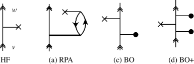
Figure 1: Dominant LCCSD contributions for the matrix elements. The double arrows represent valence state, crosses represent matrix elements $z_{ij}$ and heavy horizontal lines — cluster amplitudes. In particular, the RPA diagram involves valence doubles and BO diagram — valence singles. Here and below we do not draw the exchange variants for the diagrams.

III Generating object $C^{\dagger}C$

At this point we have reviewed application of the coupled cluster method to computing properties of univalent systems. In the remainder of this paper we deal with mathematical object

$$\left(Z_{wv}\right)_{\mathrm{conn}}=\sum_{\lambda=0}^{\infty}\sum_{\mu=0}^{\infty}\frac{1}{\lambda!\mu!}\langle 0_{c}|a_{w}S^{\dagger}_{w}(C^{\dagger})^{\lambda}\,Z\,(C)^{\mu}S_{v}a^{\dagger}_{v}|0_{c}\rangle_{\mathrm{conn}}\,.$$ (12)

As prescribed by the Wick theorem Lindgren and Morrison (1986), this expression may be simplified by contracting creation and annihilation operators between various parts of this expression. Very complex structures may arise, so as a preliminary construct, consider a product $C^{\dagger}C$. Using the Wick theorem, this product may be expanded into a sum of normal forms

$$C^{\dagger}C=\left(C^{\dagger}C\right)_{0}+\left(C^{\dagger}C\right)_{1}+\left(C^{\dagger}C\right)_{2}+\cdots=$$

$$c_{0}+\sum_{ij}c_{ij}\left\{a_{i}^{\dagger}a_{j}\right\}+\frac{1}{2}\sum_{ij}c_{ijkl}\left\{a_{i}^{\dagger}a_{j}^{\dagger}a_{l}a_{k}\right\}+\cdots$$

Here notation $\left(C^{\dagger}C\right)_{k}$ stands for $k$-body term. The zero-body term $c_{0}$ does not have any free particle or hole lines and would not contribute to connected diagrams of $Z_{wv}$. One-body term will lead to dressing of particle and hole lines, discussed in Section IV. A part of two-body term will lead to RPA-like dressing of LCCSD diagrams for matrix elements, as shown in Section IV.

IV Dressing particle and hole lines

In this section we focus on one-body term of the product $C^{\dagger}C$, Eq. (III), and derive all-order insertions for particle and hole lines. To this end it is useful to explicitly express the one-body term using particle and core labels

$$\left(C^{\dagger}C\right)_{1} = -\sum_{ab}c_{ba}a_{a}a_{b}^{\dagger}+\sum_{mn}c_{mn}a_{m}^{\dagger}a_{n}+$$ (14)

$$\sum_{ma}c_{ma}a_{m}^{\dagger}a_{a}+\sum_{ma}c_{am}a_{a}^{\dagger}a_{m}\,.$$

Topologically, the first term is an object where a free hole line enters some (possibly very complex) structure from above and another hole line leaves below. The second term has a similar structure but with particle lines. In Fig. 2, we draw these object as rectangles with “stumps” indicating where the particle or hole line is to be attached. The remaining terms in Eq. (14) have both particle and hole lines involved; we will disregard these terms in the following discussion.

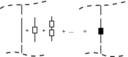
Figure 2: Schematic dressing of particle and hole lines in the CC diagrams for matrix elements.

First we prove that given a certain CC diagram for matrix elements we may “dress” all particle and hole lines as shown in Fig. 2. We start with a “seed” (“bare”) diagram coming from a certain set of contractions in Eq. (12)

$$\frac{1}{\lambda_{0}!\mu_{0}!}\langle 0_{c}|a_{w}S^{\dagger}_{w}(C^{\dagger})^{\lambda_{0}}\,Z\,(C)^{\mu_{0}}S_{v}a^{\dagger}_{v}|0_{c}\rangle_{\mathrm{seed}}\,.$$ (15)

As a next step consider a subset of terms of Eq. (12), constrained as $\lambda=\lambda_{0}+n$, $\mu=\mu_{0}+n$, $n=1,2,3,\ldots$. In these terms carry out contractions within a product of $\lambda_{0}+n$ $C^{\dagger}$ operators and $\mu_{0}+n$ $C$-operators

$$\underset{\lambda_{0}+n}{\underbrace{C^{\dagger}\cdots C^{\dagger}}}\underset{\mu_{0}+n}{~{}\underbrace{C\cdots C}}\,.$$

Within this group there are $C^{n}_{\lambda_{0}+n}\times C^{n}_{\mu_{0}+n}$ ways to pick out $n$ pairs of operators from the two sets, $C^{n}_{k}$ being binomial coefficient. Once the two strings of $n$ operators are chosen, there are $n!$ possible ways to contract into pairs $\left(C^{\dagger}C\right)_{1}$ object. Finally, we contract the $n$ resulting objects into a chain (see Fig. 2); there are $n!$ possible combinations. Combining all these factors, we recover the original factor $1/(\lambda_{0}!\mu_{0}!)$ in front of the seed diagram (15).

We may define a dressed particle-line insertion $\xi_{mn}$ in Fig. 2 as

$$\sum_{mn}\xi_{mn}a^{\dagger}_{m}a_{n}=\sum_{mn}\delta_{mn}a^{\dagger}_{m}a_{n}+\left(C^{\dagger}C\right)_{\mathrm{p-p}}+$$

$$\left(\left(C^{\dagger}C\right)_{\mathrm{p-p}}\left(C^{\dagger}C\right)_{\mathrm{p-p}}\right)_{\mathrm{p-p}}+\cdots\,,$$

where the subscript p-p denotes that we have to keep an insertion with a single incoming and a single outgoing particle line, e.g., $\left(C^{\dagger}C\right)_{\mathrm{p-p}}=\sum_{mn}c_{mn}a^{\dagger}_{m}a_{n}$. Notice the absence of numerical factors in front of terms of the series; this fact follows from the preceding discussion. Explicitly,

$$\xi_{mn}=\delta_{mn}+c_{mn}+\sum_{r}c_{mr}c_{rn}+\cdots\,.$$ (16)

This series may be generated by iteratively solving an implicit equation

$$\xi_{mn}=\delta_{mn}+\sum_{r}c_{mr}\xi_{rn}\,.$$ (17)

The very same argument holds for dressed insertions into the hole lines.

The derivation presented above can be generalized to include simultaneous dressing of all particle-hole lines of a given diagram, including the inner lines of the original “bare” object $\left(C^{\dagger}C\right)_{1}$ itself. Below we illustrate our dressing scheme in case when the cluster operator is truncated at single and double excitations.

IV.1 Singles-doubles approximation

With the truncated cluster operator the hole-line insertion reads

$$c_{ba}=\sum_{m}\rho_{mb}^{*}\rho_{ma}+\frac{1}{2}\sum_{cmn}\tilde{\rho}^{*}_{mnbc}\tilde{\rho}_{mnac}$$ (18)

and the particle-line insertion is

$$c_{mn}=-\sum_{a}\rho^{*}_{na}\rho_{ma}-\frac{1}{2}\sum_{abr}\tilde{\rho}^{*}_{nrab}\tilde{\rho}_{mrab}\,,$$ (19)

where we introduced anti-symmetric quantities $\tilde{\rho}_{mnab}=\rho_{mnab}-\rho_{nmab}$.

Diagrammatically,

$$c_{mn}a_{m}^{\dagger}a_{n}=\raisebox{-21.52771pt}{\includegraphics[scale={0.4}]{dressed_line_skewed.eps}}\,.$$

As discussed in the first part of this Section, we may dress all the particle/hole lines according to the all-order scheme in Fig. 3.

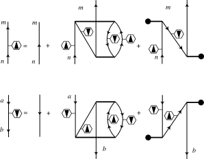
Figure 3: Dressing of particle and hole lines in the singles-doubles approximation. The upper and lower panels represent dressing of particle and hole lines respectively.

Algebraically,

$$\xi_{mn} = \delta_{mn}-\sum_{a}\rho_{ma}R_{na}^{\ast}-\sum_{abr}\tilde{\rho}_{mrab}R_{nrab}^{\ast}\,,$$ (20)

$$\xi_{ba} = \delta_{ba}-\sum_{m}\rho_{mb}^{\ast}R_{ma}-\sum_{mnc}\tilde{\rho}_{mnbc}^{\ast}R_{mnac}\,,$$

where we introduced dressed core cluster amplitudes

$$R_{na}^{\ast} = \sum_{b}\xi_{ba}\sum_{s}\rho_{sb}^{\ast}\xi_{sn}\,,$$

$$R_{nrab}^{\ast} = \sum_{t}\xi_{rt}\sum_{s}\xi_{ns}\sum_{c}\xi_{ca}\sum_{d}\rho_{stcd}^{\ast}\xi_{db}\,.$$ (21)

We solve Eq. (20) iteratively

$$\xi_{mn}^{\left(i+1\right)} = \delta_{mn}-\sum_{a}\rho_{ma}R_{na}^{\left(i\right)\ast}-\sum_{abr}\tilde{\rho}_{mrab}R_{nrab}^{\left(i\right)\ast}\ ,$$

$$\xi_{ba}^{\left(i+1\right)} = \delta_{ba}-\sum_{m}\rho_{mb}^{\ast}R_{ma}^{\left(i\right)}-\sum_{mnc}\tilde{\rho}_{mnbc}^{\ast}R_{mnac}^{\left(i\right)},$$ (22)

where the dressed amplitudes $R_{\cdots}^{(i)}$ are to be computed with coefficients $\xi_{\cdots}^{(i)}$ obtained at the previous step.

With the calculated insertions $\xi$ we can “upgrade” the LCCSD diagrams (compare Fig. 1 and Fig. 4). To this end we introduce dressed matrix elements $\bar{z}_{ij}$ and dressed valence cluster amplitudes $R_{mv}$ and $R_{mnva}$, similar to Eq. (21)

$$\bar{z}_{mn} = \sum_{rs}\xi_{mr}z_{rs}\xi_{sn}\,,$$

$$\bar{z}_{ab} = \sum_{cd}\xi_{ca}z_{cd}\xi_{db}\,,$$ (23)

$$R_{mv} = \sum_{n}\xi_{mn}\rho_{nv}\,,$$

$$R_{mnva} = \sum_{brs}\xi_{nr}\xi_{ba}\xi_{sm}\rho_{srvb}\,.$$ (24)

Notice that the incoming valence line in the valence amplitudes $\rho_{mnav}$ and $\rho_{mv}$ is not dressed, since it does not represent a free end. With these objects we may dress the LCCSD diagrams, as shown in Fig. 4.

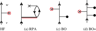
Figure 4: Dressing of particle-hole lines in the dominant LCCSD diagrams, Fig. 1. The circled crosses represent line-dressed matrix elements, Eq. (23), and the double-lined valence cluster amplitude is the dressed amplitude, Eq. (24).

Numerically, we rigorously computed the four dressed diagrams shown in Fig. 4. In the remaining LCCSD diagrams, listed in Ref. Blundell et al. (1989), we have replaced the bare matrix elements with the dressed matrix elements, Eq. (23). Notice that the dressing of the Hartree-Fock diagram subsumes LCCSD diagrams

$$Z^{(\mathrm{g})}_{wv} = -\sum_{ma}\rho_{ma}^{*}\rho_{wa}z_{mv}+\mathrm{h.c.s.}\,,$$

$$Z^{(\mathrm{t})}_{wv} = -\sum_{mnab}\rho_{mnba}^{*}\tilde{\rho}_{nwab}z_{mv}+\mathrm{h.c.s.}\,.$$ (25)

from Ref. Blundell et al. (1989), so that these diagrams are to be discarded in the present approach. We postpone discussion of numerical results until Section VII.

V RPA-like dressing

In this Section we continue with the systematic dressing of the coupled-cluster diagrams for matrix elements based on the topological structure of the product $C^{\dagger}C$, Eq. (III). Here we focus on the two-body term of this object. The insertion that generates the RPA-like chain of diagrams is due to a two-particle/two-hole part of the object $\left(C^{\dagger}C\right)$,

$$\left(C^{\dagger}C\right)_{\mathrm{RPA}}\equiv\sum_{mnab}\tilde{c}_{nbma}~{}\left\{a_{n}^{\dagger}a_{b}^{\dagger}a_{a}a_{m}\right\}\,,$$ (26)

where we used a symmetry property $c_{ijkl}=c_{jilk}$, and $\tilde{c}_{ijkl}=c_{ijkl}-c_{ijlk}$. An analysis identical to that presented for line dressing in Section IV leads us to introducing an RPA-dressed object $\mathcal{T}_{nbma}$,

$$\sum_{mnab}\tilde{\mathcal{T}}_{nbma}\left\{a_{n}^{\dagger}a_{b}^{\dagger}a_{a}a_{m}\right\}=-\sum_{mnab}\delta_{mn}\delta_{ab}\left\{a_{n}^{\dagger}a_{b}^{\dagger}a_{a}a_{m}\right\}$$

$$+ \left(C^{\dagger}C\right)_{\mathrm{RPA}}+\left(\left(C^{\dagger}C\right)_{\mathrm{RPA}}\left(C^{\dagger}C\right)_{\mathrm{RPA}}\right)_{\mathrm{RPA}}+\cdots\,,$$

where subscript RPA specifies that the objects inside the brackets are to be contracted so that the result has the same free particle/hole ends as the original bare object $\left(C^{\dagger}C\right)_{\mathrm{RPA}}$, Eq. (26). The sign of the leading term (with the Kronecker symbols) is chosen in such a way that a product of this term with a particle-hole object like $z_{rc}a_{c}a^{\dagger}_{r}$ results in the original object.

A detailed consideration leads to an implicit equation for the RPA-dressed particle-hole insertion

$$\tilde{\mathcal{T}}_{nbma}=-\delta_{mn}\delta_{ab}-\sum_{rc}\tilde{c}_{ncra}\tilde{\mathcal{T}}_{rbmc}\,.$$ (28)

This equation, presented graphically in Fig. 5, can be solved iteratively.

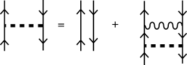
Figure 5: Graphical equation for RPA-dressed insertion. The dashed horizontal line is the dressed insertion $\mathcal{T}_{nbma}$, while the bare object $c_{nbma}$ is represented by a wavy line.

The resulting insertion $\mathcal{T}_{nbma}$ may dress any particle-hole vertex of a diagram as shown in Fig. 6.

Figure 6: Dressing particle-hole vertex of a diagram with the RPA insertion, Fig. 5.

As an example, consider dressing of particle-hole matrix elements of operator $Z$: $z_{ma}a^{\dagger}_{m}a_{a}$. The equation for the dressed matrix element $\bar{z}_{ma}$ may be derived simply as

$$\bar{z}_{ma}^{\mathrm{RPA}} \equiv -\sum_{nb}\tilde{\mathcal{T}}_{mbna}z_{nb}\,,$$

$$\bar{z}_{ma}^{\mathrm{RPA}} = z_{ma}+\sum_{rc}\tilde{c}_{mcra}\sum_{nb}\tilde{\mathcal{T}}_{rbnc}z_{nb}=z_{ma}-\sum_{nb}\tilde{c}_{mbna}\bar{z}_{nb}^{\mathrm{RPA}}\,,$$

where we used Eq. (28) for the dressed object $\tilde{\mathcal{T}}_{mbna}$. Finally we obtain a set of two equations

$$\bar{z}_{am}^{\mathrm{RPA}} = z_{am}-\sum_{nb}\tilde{c}_{mbna}^{*}\bar{z}_{bn}^{\mathrm{RPA}}\,,$$

$$\bar{z}_{ma}^{\mathrm{RPA}} = z_{ma}-\sum_{nb}\tilde{c}_{mbna}\bar{z}_{nb}^{\mathrm{RPA}}\,.$$

The resulting equations resemble the traditional RPA formulae for dressed matrix elements (see, e.g., Ref. Johnson et al. (1996)), but do not couple $\bar{z}_{am}^{\mathrm{RPA}}$ and $\bar{z}_{ma}^{\mathrm{RPA}}$. In addition, the role of the residual Coulomb interaction of the traditional RPA formulae is played by the matrix elements of $\left(C^{\dagger}C\right)_{\mathrm{RPA}}$ object (that is dominated by second order in the Coulomb interaction, see Section VI). In addition, we would like to emphasize that the line-dressed matrix elements, Eq. (23) also include matrix elements between core and virtual orbitals; these are to be distinguished from the RPA-like matrix elements, Eq. (V).

The above derivation is only valid when dressing a single isolated vertex. More complex situation arises whenever a horizontal cross-cut through a diagram produces several (not just two, as in Fig. 6) unquenched particle and hole lines. Then the lower particle and hole lines of the object $\left(C^{\dagger}C\right)_{\mathrm{RPA}}$ could be attached to the unquenched lines of the bare diagram in any order and “cross-dressing” may occur. As an illustration, consider RPA-dressing of the valence double contribution to the wavefunction $\sum_{mna}\rho_{mnva}a^{\dagger}_{m}a^{\dagger}_{n}a_{a}$. It arises, for example, when the diagram $Z^{(a)}_{wv}$ (see Fig. 1(a)) is cut across horizontally. The valence double contains two equivalent vertexes $a^{\dagger}_{m}a_{a}$ and $a^{\dagger}_{n}a_{a}$. First we may attach the RPA object to the $m-a$ vertex and at the second step to the $n-a$ vertex. Apparently, this scenario is not covered by Eq. (V), since it implies that all RPA insertions are attached to the same vertex. Nevertheless, the RPA-like dressing can be carried out in a straightforward fashion. To continue with the illustration, the RPA-dressed valence double amplitude may be defined as follows (compare to Eq. (V) )

$$\sum_{mna}\mathcal{R}_{mnva}^{\mathrm{RPA}}a^{\dagger}_{m}a^{\dagger}_{n}a_{a} = \left(\left[1+\left(C^{\dagger}C\right)_{\mathrm{RPA}}+\left(\left(C^{\dagger}C\right)_{\mathrm{RPA}}\left(C^{\dagger}C\right)_{\mathrm{RPA}}\right)_{\mathrm{RPA}}+\cdots\right]\times\right.$$ (29)

$$\left.\sum_{mna}\rho_{mnva}a^{\dagger}_{m}a^{\dagger}_{n}a_{a}\right)_{\mathrm{val.double}}\,.$$

Here subscript “val. double” indicates that we select a contribution having the same free ends as the R.H.S. of the equation. The numerical factors in front of the individual RPA contributions are derived similarly to the line-dressing factors (see Section IV). Explicitly, we deal with a chain of diagrams

$$\mathcal{R}_{mnva}^{\mathrm{RPA}}=\rho_{mnva}-\sum_{br}\tilde{c}_{nbra}\tilde{\rho}_{mrvb}+$$ (30)

$$\sum_{bcrs}\left(\tilde{c}_{ncsa}\tilde{c}_{sbrc}\tilde{\rho}_{mrvb}-\tilde{c}_{ncsa}\tilde{c}_{mbrc}\tilde{\rho}_{srvb}\right)+\cdots\,.$$

Examining the structure of the above expression we finally arrive at

$$\mathcal{R}_{mnva}^{\mathrm{RPA}}=\rho_{mnva}-\sum_{sb}\tilde{c}_{nbsa}\tilde{\mathcal{R}}_{msvb}^{\mathrm{RPA}}\,,$$ (31)

i.e., we have demonstrated how to dress the valence doubles. This example can be easily generalized to several equivalent vertexes: the Eq. (29) has to be rewritten using as the seed object the underlying structure of the unquenched lines produced by a horizontal cross-cut through a diagram.

V.1 Singles-doubles approximation

Now we specialize our discussion of the RPA-like dressing to the cluster operator truncated at single and double excitations. In this CCSD approximation we obtain for the bare RPA-like insertion

$$\tilde{c}_{nbma}\approx-\rho_{mb}^{*}\rho_{na}-\sum_{rc}\tilde{\rho}_{mrbc}^{\ast}\tilde{\rho}_{nrac}\,.$$ (32)

Notice that one has to be careful when dealing with the first (singles $\times$ singles) term; it is represented by a disconnected diagram and may produce undesirable disconnected diagrams for matrix elements, Eq. (10).

By substituting the CCSD insertion, Eq.(32), into Eq. (V) and Eq. (31), we immediately derive expressions for the dressed matrix elements and the RPA-dressed valence doubles. For example,

$$\mathcal{R}_{mnva}^{\mathrm{RPA}} = \rho_{mnva}+\sum_{sb}\left(\sum_{rc}\tilde{\rho}_{nrac}\tilde{\rho}_{srbc}^{\ast}\right)\tilde{\mathcal{R}}_{msvb}^{\mathrm{RPA}}\,,$$ (33)

$$\bar{z}_{ma}^{\mathrm{RPA}} = z_{ma}+\sum_{nb}\left(\sum_{rc}\tilde{\rho}_{nrbc}^{\ast}\tilde{\rho}_{mrac}\right)\bar{z}_{nb}^{\mathrm{RPA}}\,.$$ (34)

Here we omitted a small contribution to $\tilde{c}_{nbma}$, Eq. (32), from the product of core singles. As discussed in Section VI this contribution would arise in the higher orders (sixth order) of MBPT.

Practically, we notice that among the dominant LCCSD diagrams shown in Fig. 1, the particle-hole vertex occurs only in the RPA diagram $Z_{wv}^{(a)}$. Focusing on this particular diagram, the “upgraded” $Z_{wv}^{(a)}$ is simply

$$\left(Z^{(\mathrm{a})}_{wv}\right)_{\mathrm{dress}}=\sum_{ma}z_{am}\tilde{\mathcal{R}}_{wmva}^{\mathrm{RPA}}+\mathrm{h.c.s.}\,.$$ (35)

Notice that the use of the RPA-dressed matrix elements to upgrade the $Z_{wv}^{(a)}$ diagram, such as

$$\left(Z^{(\mathrm{a})}_{wv}\right)_{\mathrm{mel.\,dress}}=\sum_{ma}\bar{z}_{am}^{\mathrm{RPA}}\tilde{\rho}_{wmva}+\mathrm{h.c.s.}\,$$ (36)

does not lead to the identical result, because it misses dressing of the $w-a$ vertex. Moreover, we found numerically that dressing of both vertexes, as in more general Eq. (35), is equally important.

Finally, it is worth noting that with the RPA-like dressing scheme proposed here, the CCSD calculations would recover the entire chain of RPA diagrams. However, if the calculations of the wavefunctions are done using the linearized version of the coupled-cluster equations (as in Refs. Blundell et al. (1989, 1991); Safronova et al. (1998, 1999)), a part of the RPA diagrams would still be missing Blundell et al. (1989). To summarize, the inclusion of the CCSD non-linear terms in the CC equations is crucial for a fully consistent treatment of the RPA sequence.

VI Comparison with the IV-order diagrams

Coupled cluster method can be straightforwardly connected with the direct order-by-order many-body perturbation theory. In particular, for univalent systems, when the calculations are carried out starting from the frozen-core Hartree-Fock potential, the lowest-order contributions to the double excitation cluster amplitudes are

$$\rho_{mnva} \approx -\frac{g_{mnva}}{\varepsilon_{m}+\varepsilon_{n}-\varepsilon_{a}-\varepsilon_{v}}\,,$$

$$\rho_{mnab} \approx -\frac{g_{mnab}}{\varepsilon_{m}+\varepsilon_{n}-\varepsilon_{a}-\varepsilon_{b}}\,.$$ (37)

Here $g_{ijkl}$ is the matrix element of the residual (beyond the HF potential) Coulomb interaction between the electrons. It can be shown that while the LCCSD method recovers all third-order diagrams for matrix elements, it starts missing diagrams in the fourth order of MBPT. Our group has investigated these 1,648 complementary IVth order diagrams in Refs. Derevianko and Emmons (2002); Cannon and Derevianko (2004). Among the diagrams complementary to LCCSD matrix element contributions, there are seven terms (class $Z_{1\times 2}\left(D_{nl}\right)$ in Ref. Derevianko and Emmons (2002) ) due to non-linear terms in the expansion of the CCSD wavefunctions. Namely these $Z_{1\times 2}\left(D_{nl}\right)$ diagrams provide the lowest-order approximation for the dressing scheme proposed here.

In Fig. 7 we explore the topological structure of the $Z_{1\times 2}\left(D_{nl}\right)$ diagrams. All these diagrams come from various ways of lowest-order dressing of $Z^{(\mathrm{a})}_{wv}$ diagram, Eq. (11). A comparison shows that the present dressing approach recovers five (three line-dressed and two RPA-dressed) out of seven IVth-order diagrams. The missing diagrams are shown in the bottom row of Fig. 7, and we call them “stretched” and “ladder” diagrams, the names being derived from the structure of the highlighted dressing insertions. While the ladder diagram comes from the untreated two-body contribution to $C^{\dagger}C$ object, Eq. (III), the stretched diagram involves more complex three-body contribution to $C^{\dagger}C$. Dressing with these two insertions can be carried out in a way similar to the line- and RPA-like dressing schemes discussed in this paper and is beyond the scope of the present analysis.

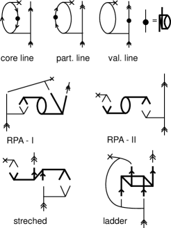
Figure 7: Topological structure of fourth-order diagrams of class $Z_{1\times 2}\left(D_{nl}\right)$ derived in Ref. Derevianko and Emmons (2002). In these diagrams horizonal lines denote Coulomb interaction and the topological objects coming from the lowest-order approximation to $C^{\dagger}C$ are highlighted. The upper three diagrams arise in the leading order of the line-dressing scheme and two diagrams in the middle are related to the RPA-dressing scheme.

We verified that in the lowest-order MBPT approximation, Eq. (37), our dressing formulae reproduce the pertinent IVth-order expressions, explicitly presented in Ref. Derevianko and Emmons (2002). Furthermore, in Table 1 we list numerical values for individual contributions to magnetic-dipole hyperfine structure constant (HFS) $A$ for ground state of ¹³³Cs and E1 transition amplitude for the principal $6p_{1/2}-6s_{1/2}$ transition in Cs. Analyzing this Table we conclude that both line– and RPA–like dressing are equally important. Moreover, for these two particular matrix elements there is a partial cancelation between the line– and RPA– dressed diagrams, so that were one of the dressings omitted, the result would be misleading. We also observe that the untreated “ladder” diagram contributes a negligibly small fraction of the total. At the same time the size of the untreated “stretched” diagram indicates that (at least for the HFS constant) it is as important as the RPA-like and line-dressed diagrams.

As to the numerics, the IVth-order calculations have been carried out using relativistic B-spline basis sets as described in Ref. Johnson et al. (1988). We used a basis set of 25 out of 30 positive-energy ($\varepsilon_{i}>-m_{e}c^{2}$) pseudo-eigenfunctions for each partial wave. Partial waves $s_{1/2}-g_{9/2}$ were included in the basis. The summation over intermediate core orbitals was limited to eight highest energy core orbitals for the E1 amplitude and included all core orbitals for the HFS constant. The reader is referred to paper Cannon and Derevianko (2004) for a description of our IVth-order code.

Type	$A(6s)$, MHz	$\langle 6s_{1/2}||D||6p_{1/2}\rangle,\mathrm{a.u.}$
core line	$-2.0$	$7.0[-3]$
particle line	$-0.90$	$2.5[-3]$
valence line	$-0.92$	$0.2[-3]$
RPA-I	$0.005$	$-9.3[-3]$
RPA-II	$4.8$	$-0.05[-3]$
stretched	$-3.0$	$0.1[-3]$
ladder	$0.05$	$-0.008[-3]$
Total	$-1.9$	$0.41[-3]$

Table 1: Breakdown of contributions to $Z_{1\times 2}(D_{nl})$ class of diagrams for the hyperfine-structure (HFS) constant $A$ for the $6s_{1/2}$ state and $6s_{1/2}-6p_{1/2}$ electric-dipole transition amplitude for ¹³³Cs atom. The lowest-order DHF values are 1425.29 MHz for the HFS constant and 5.278 a.u. for the transition amplitude. Notation $x[y]$ stands for $x\times 10^{y}$.

We verified that numerical results for dressed all-order LCCSD diagrams (see Section VI) are consistent with the values for the pertinent IVth-order diagrams. As an example consider contributions to $A(6s)$ HFS constant. Line-dressing modifies the LCCSD $Z^{(\mathrm{a})}_{wv}$ diagram by $-4.3$ MHz in a good agreement with a value of $-3.8$ MHz, the sum of the first three corresponding IVth-order diagrams from Table 1. Similarly, RPA-like dressing modifies the $Z^{(\mathrm{a})}_{wv}$ diagram by $+4.4$ MHz, while the sum of IVth-order RPA diagram from Table 1 is $4.8$ MHz.

VII Numerical results and discussion

To reiterate discussion so far, we have developed the formalism of line- and RPA-like dressing of the coupled-cluster diagrams for matrix elements. Further, we reduced our general formalism to the case when the cluster operator is truncated at single and double excitation amplitudes. We have also verified that in the lowest order we recover the relevant fourth-order diagrams both analytically and numerically. In this Section we illustrate our all-order dressing formalism with numerical results.

We have carried out relativistic calculations of the hyperfine-structure (HFS) constant $A$ for the $6s_{1/2}$ state and $6s_{1/2}-6p_{1/2}$ electric-dipole transition amplitude for ¹³³Cs atom. It is worth noting that matrix elements of hyperfine interaction and electric dipole operator allow one to access the quality of ab initio wavefunctions both close to the nucleus and at intermediate values of electronic coordinate. Such a test is essential for estimates of theoretical uncertainties of calculations of parity-nonconserving (PNC) amplitudes. The ab initio PNC amplitudes are key for high-accuracy probes of new physics beyond the standard model of elementary particles with atomic parity violation.

The results of calculations are presented in Tables 2 and 3. In these tables we augment results of the previous all-order calculations Safronova et al. (1999) with two types of new contributions: (i) all-order RPA- and line- dressing, outlined in Sections IV and V, and (ii) complementary fourth-order contributions, so that the results are complete through the fourth-order perturbation theory. Also, for the HFS constant, we incorporate the most recent values of the Breit and radiative corrections Derevianko (2002); Sapirstein and Cheng (2003).

Contribution	Value (MHz)
DHF	$1425.29$
LCCSDpT, Coulomb	$2283.1$
Breit Derevianko (2002)	$4.6$
VP+SE Sapirstein and Cheng (2003)	$-9.7$
LCCSDpT Reference	$2278.0$
Dressing
$\Delta$(line-dress)	$-11.0$
$\Delta$(RPA-dress)	$4.4$
Dressing total	$-6.7$
Complementary IVth-order
Triples	$+17.7$
$Z_{0\times 3}(D_{nl})$	$-5.5$
$Z_{1\times 2}\left(D_{\mathrm{nl}}\right)$, stretched	$-3.0$
$Z_{1\times 2}\left(D_{\mathrm{nl}}\right)$, ladder	$+0.1$
$\Delta$(ZIV) total	$+9.3$
Final ab initio	$2280.6$
Experiment	$2298.2$

Table 2: Contributions to the magnetic-dipole hyperfine-structure constant $A$ of the ground $6s_{1/2}$ state of ¹³³Cs.

Contribution	Value (a.u.)
DHF	$5.278$
LCCSDSafronova et al. (1999)	$4.482$
LCCSDpT Reference	$4.558$
Dressing
$\Delta$(line-dress)	$0.008$
$\Delta$(RPA-dress)	$-0.007$
Dressing corr. total	$-0.001$
Complementary IVth-order
Triples	$-0.043$
$Z_{0\times 3}(D_{nl})$	$0.014$
$Z_{1\times 2}\left(D_{\mathrm{nl}}\right)$, stretched	$1.0[-4]$
$Z_{1\times 2}\left(D_{\mathrm{nl}}\right)$, ladder	$-8.6[-6]$
$\Delta$(ZIV) total	$-0.029$
Final ab initio	$4.528$
Experiment
Young et al. (1994)	$4.5097(45)$
Rafac et al. (1999)	$4.4890(65)$
Derevianko and Porsev (2002)	$4.5064(47)$
Amiot et al. (2002)	$4.5006(13)$
Amini and Gould (2003)	$4.510(4)$

Table 3: Contributions to $\langle 6s_{1/2}||D||6p_{1/2}\rangle$ electric-dipole matrix element for Cs atom.

LCCSDpT (perturbative triples) approximation. We depart from the results of the coupled-cluster calculation described in Ref. Safronova et al. (1999). These are linearized coupled-cluster calculations, with the wavefunctions truncated at single and double excitations from the reference Slater determinant. In addition, following Ref. Blundell et al. (1991), the perturbative effect of triple excitations has been incorporated into the singles-doubles equation (LCCSDpT method). The main consequence of this perturbative treatment is that the resulting valence removal energies are complete through the third order of perturbation energies. There is also a substantial (a few per cent for Cs) improvement in the accuracy of the resulting LCCSDpT hyperfine constants over the LCCSD values. At the same time the theory-experiment agreement for the E1 amplitudes significantly degrades (see Table 3): while the LCCSD amplitudes differ by 0.4% from 0.03%-accurate experimental data Amiot et al. (2002), the more sophisticated LCCSDpT matrix elements deviate from measurements by as much as 1.3%. In other words, both LCCSD and LCCSDpT methods are poorly suited for calculating parity-non-conserving (PNC) amplitudes in ¹³³Cs with uncertainty of a few 0.1%. It is one of the goals of this paper to establish a method that would provide a consistent accuracy for both HFS constants and dipole matrix elements (and thus PNC amplitudes).

Procedure. First we solved the relativistic LCCSDpT equations, as described in Ref. Safronova et al. (1999). With the computed cluster amplitudes we calculated LCCSDpT matrix elements and recovered results published in Ref. Safronova et al. (1999). Further, we solved the line-dressing equations (22) and computed the line-dressed cluster amplitudes and matrix elements. The convergence rate was fast: four iterations were sufficient to stabilize the norms of the line-dressed cluster amplitudes at a level of a few parts per million. Finally, we solved the iterative equation for the RPA-dressed valence amplitudes, Eq.(33). It turned out to be very computationally intensive part of the scheme and we iterated the equations only once. We used the computed RPA-dressed valence amplitudes in calculations of the dominant diagram $Z^{(a)}_{wv}$, see Eq. (35). In the remaining diagrams that involve particle-hole matrix elements, we employed RPA-dressed matrix elements $\bar{z}^{\mathrm{RPA}}_{ij}$. A numerical iterative solution of equations for $\bar{z}^{\mathrm{RPA}}_{ij}$, Eq. (34) required only a few iterations to converge to seven significant figures.

Line dressing. In Table 4 we illustrate the importance of line dressing; in this table we present differences between line-dressed and bare LCCSDpT diagrams for the the hyperfine constant and E1 amplitude. The dressing of the leading order HF diagram subsumes the LCCSD diagrams $Z^{(\mathrm{g})}_{wv}$ and $Z^{(\mathrm{t})}_{wv}$, Eq. (25). A direct calculation of these diagrams results in $Z^{(\mathrm{g})}_{wv}+Z^{(\mathrm{t})}_{wv}=-22.9$ MHz for $A(6s)$ and $-1.75\times 10^{-3}$ a.u. for the E1 amplitude. These values are consistent with dressing-induced modifications of the HF diagram ($-22.0$ MHz and $-1.7\times 10^{-3}$ a.u., respectively) from Table 4. The modifications of the $Z^{(\mathrm{a})}_{wv}$ diagram are consistent with the values of the pertinent fourth-order diagrams, see Section VI and Table 1. A large dressing correction for HFS constant comes from the diagram $Z^{(\mathrm{c})}_{wv}$; it is nominally a fifth-order diagram. The relative importance of this diagram is not surprising since it is based upon Brueckner orbitals (self-energy or core polarization effect). As for the E1 amplitude, the line-dressing correction is dominated by $Z^{(\mathrm{a})}_{wv}$; i.e., it is dominated by the fourth-order contribution. For the HFS constant, a relative smallness of the line-dressing correction to $Z^{(\mathrm{a})}_{wv}$ diagram arises due to a delicate cancelation of relatively large contributions from dressing of the core, particle and valence lines of the diagram (see Table 1). Finally, in the bottom line of the Table 4 we present a difference between the line-dressed (all diagrams) and bare values. The dressing of the HF diagram plays a negligible role here, since it is dominated by the diagrams already included in the LCCSDpT values. The line dressing contributes at a sizable 0.5% level to the HFS constant and at 0.2% level to the E1 amplitude.

Type	$A(6s)$, MHz	$\langle 6s_{1/2}||D||6p_{1/2}\rangle,\mathrm{a.u.}$
$Z^{(\mathrm{HF})}_{wv}$	$-22$	$-1.7[-3]$
$Z^{(\mathrm{a})}_{wv}$	$0.04$	$9.3[-3]$
$Z^{(\mathrm{c})}_{wv}$	$-8.6$	$-0.5[-3]$
$Z^{(\mathrm{d})}_{wv}$	$-0.8$	$-3.6[-5]$
All diagrams	$-11$	$8.0[-3]$

Table 4: Line-dressing induced modifications to dominant LCCSDpT diagrams, Eq. (11), for the HFS constant $A$ for the $6s_{1/2}$ state and $6s_{1/2}-6p_{1/2}$ E1 transition amplitude for ¹³³Cs atom.

RPA-like dressing. Numerically dominant contribution due to the RPA-like dressing arises for $Z^{(\mathrm{a})}_{wv}$ diagram, where we used RPA-dressed valence amplitudes. The induced correction is as large as 0.2% for both dipole amplitude and HFS constant. The dressing of particle-hole matrix elements ($z_{ij}\rightarrow\bar{z}^{\mathrm{RPA}}_{ij}$) in diagrams beyond $Z^{(\mathrm{a})}_{wv}$ played a relatively minor role, contributing at a level of only 0.01% for both test cases.

Complementary fourth-order diagrams. The LCCSDpT method misses certain many-body diagrams for matrix elements starting from the fourth-order of MBPT. These complementary corrections in the fourth order come from triple and disconnected quadruple (or nonlinear double) excitations. In Ref. Derevianko and Emmons (2002) these corrections were classified by the role of triples and disconnected quadruples in the matrix elements (i) an indirect effect of triples and disconnected quadruples on single and double excitations lumped into class $Z_{0\times 3}$; (ii) direct contribution to matrix elements, $Z_{1\times 2}$; (iii) corrections to normalization, $Z_{\mathrm{norm}}$. More refined classification reads

$$\left(Z^{(4)}_{wv}\right)_{\mathrm{non-LCCSD}}=Z_{1\times 2}(T_{v})+Z_{1\times 2}(T_{c})+$$

$$Z_{0\times 3}(S_{v}[T_{v}])+Z_{0\times 3}(D_{v}[T_{v}])+$$

$$Z_{0\times 3}(S_{c}[T_{c}])+Z_{0\times 3}(D_{v}[T_{c}])+$$

$$Z_{1\times 2}\left(D_{\mathrm{n}l}\right)+Z_{0\times 3}\left(D_{\mathrm{n}l}\right)+Z_{\mathrm{norm}}(T_{v})\,.$$

Here we distinguished between valence ($T_{v}$) and core ($T_{c}$) triples and introduced a similar notation for singles ($S$) and doubles ($D$). Notation like $D_{v}[T_{c}]$ stands for effect of core triples ($T_{c}$) on valence doubles $D_{v}$ through an equation for valence doubles. The LCCSDpT method combines several diagrams from $Z_{1\times 2}(T_{v})$ and $Z_{0\times 3}(S_{v}[T_{v}])$ classes. We removed these already included diagrams from the fourth-order triples in Tables 2 and 3. Diagrams $D_{\mathrm{nl}}$ are contributions of disconnected quadruples. As discussed in Section VI namely one of such contributions, $Z_{1\times 2}\left(D_{\mathrm{n}l}\right)$, provides the lowest-order approximation to our all-order dressing scheme. In Tables 2 and 3 we added the contributions of untreated “stretched” and “ladder” diagrams of the $Z_{1\times 2}\left(D_{\mathrm{n}l}\right)$ class and also from $Z_{0\times 3}\left(D_{\mathrm{n}l}\right)$ class. The latter contribution would have been accounted for by solving the full (not linearized) CC equations. In our large-scale fourth-order calculations we have employed the code described in Ref. Cannon and Derevianko (2004); all the formulas for a large number of diagrams and the code have been generated automatically using symbolic algebra tools. While the resulting fourth-order corrections from triples are at the level of 1%, we notice that there are certain noticeable cancelations between various diagrams. Thus a complete all-order treatment of triples would be essential for attaining the next level of theoretical accuracy.

Hyperfine constant results. Details of calculation of the hyperfine constant $A(6s_{1/2})$ are presented in Table 2. To clarify the role of correlations, we first incorporate a number of small but important effects into the reference value: Bohr-Weiskopf effect, Breit and radiative corrections. The “LCCSDpT, Coulomb” value has been computed using the finite nuclear size, both for determination of wavefunctions and computing matrix elements of hyperfine interaction (this accounts for 0.5%.) We also include Breit corrections from Ref. Derevianko (2002); these corrections differ substantially from those incorporated in Ref. Safronova et al. (1999); Blundell et al. (1991) due to order-of-magnitude important correlation corrections. Finally, radiative corrections to magnetic-dipole hyperfine-structure constants for the ground state of alkali-metal atoms were computed recently by Sapirstein and Cheng (2003). They found that the vacuum polarization and self-energy (VP+SE) contribute as much as 0.4% to the ab initio value. The reader should be careful with adopting Breit values from Ref.Sapirstein and Cheng (2003), because these values do not include correlation corrections (see Ref. Derevianko (2002) and references therein). The final value, marked as “LCCSDpT Reference” deviates by 0.9% from (exact) experimental value.

Dressing corrections partially cancel, resulting in 0.3% total dressing contribution. Fourth-order diagrams, complementary to those already included in the LCCSDpT value are dominated by a contribution due to triple excitations (0.8%). We also include the “stretched” and “ladder” IV-order diagrams missed by our dressing scheme (see Section VI). Almost all the correlation corrections are of similar sizes but of different signs, so the dressing and IV-th order corrections cancel, so that the final correlation correction is only 0.1%, just slightly improving the theory-experiment agreement when compared with the “LCCSDpT Reference” value. Our ab initio value for the HFS constant deviates by 0.8% from the experimental value.

Electric-dipole $6s_{1/2}-6p_{1/2}$ transition amplitude. Details of calculation for the dipole matrix element are compiled in Table 3. We do not include Breit and radiative corrections in that Table, since the Breit interaction contributes only 0.02% to this matrix element Derevianko (2002), and radiative corrections are not known from the literature.

There were several high-accuracy experimental determinations of $\langle 6p_{1/2}||D||6s_{1/2}\rangle$ matrix element. We list these matrix elements in the bottom of Table 3. In Refs. Young et al. (1994); Rafac et al. (1999) this matrix element has been extracted from the measured lifetime of the $6p_{1/2}$ state. Determination of Ref. Amiot et al. (2002) is based on photoassociative spectroscopy of cold Cs atoms (i.e., inferred from high-accuracy measurement of molecular potentials). Another approach to extraction of dipole matrix elements has been proposed by us in Ref. Derevianko and Porsev (2002): we exploited an enhanced sensitivity of static electric-dipole polarizability $\alpha(0)$ of the ground state and van der Waals coefficient $C_{6}$ of the ground molecular state to the matrix elements of principal transitions $\langle 6p_{3/2}||D||6s_{1/2}\rangle$ and $\langle 6p_{1/2}||D||6s_{1/2}\rangle$. Essential to the extraction of individual matrix elements was a high-accuracy ratio of these two dipole matrix elements measured in Ref. Rafac and Tanner (1998). Based on the proposed method Derevianko and Porsev (2002), the $\langle 6p_{1/2}||D||6s_{1/2}\rangle$ matrix element has been deduced from high-accuracy $C_{6}$ in Ref. Derevianko and Porsev (2002) and in Ref. Amini and Gould (2003) it has been inferred from $\alpha(0)$ measured in that work. The most accurate matrix element comes from photoassociation spectroscopy Amiot et al. (2002); their result has 0.03% accuracy and we will use that value below for calibrating ab initio calculations.

The reference LCCSDpT E1 matrix element deviates from high-accuracy measurements by as much as 1.3%. The correlation corrections (dressing and fourth-order) computed by us improve the agreement to about 0.6% , i.e., the ab initio accuracy becomes comparable to that for the HFS constant. An analysis of Table 3 shows that due to cancelation of line- and RPA-like-dressing corrections the overall effect of dressing is negligible for this transition amplitude. At the same time, the forth-order corrections due to triple excitations beyond LCCSDpT triples are very large, almost 1%. There corrections due to residual fourth-order RPA corrections ($Z_{0\times 3}(D_{nl})$) are also sizable, and tend to decrease the effect of triples. Our forth-order calculation demonstrates that a full (beyond that of LCCSDpT) treatment of triple excitations improves the accuracy of ab initio transition amplitudes.

VIII Conclusion

The main two results of this work are: (i) development and application of all-order dressing formalism for matrix elements computed with coupled-cluster method; (ii) first calculations of matrix elements for Cs complete through the fourth order of many-body perturbation theory.

To reiterate, our dressing formalism is built upon a hierarchical expansion of the product of clusters $C^{\dagger}C$ into a sum of $n$-body insertions. We considered two types of insertions: particle/hole line insertion coming from the one-body part of the product and two-particle/two-hole RPA-like insertion due to the two-body part. We demonstrated how to “dress” these insertions and formulated iterative equations. Particular attention has been paid to the singles-doubles truncation of the full cluster operator and we derived the dressing equations for this popular approximation. We have upgraded coupled-cluster diagrams for matrix elements with the dressed insertions for univalent systems and highlighted a relation to pertinent fourth-order diagrams. Finally, we illustrated our formalism with relativistic calculations for Cs atom.

Our relativistic calculations also include a large number of fourth-order diagrams complementary to LCCSDpT method (Linearized Coupled-Cluster Single-Doubles method with perturbative treatment of Triples; it is the most sophisticated CC approximation applied in relativistic calculations for Cs so far). The resulting analysis is complete through the fourth-order of many-body perturbation theory. We find that these complementary diagrams substantially improve the theory-experiment agreement for an important electric-dipole $6s_{1/2}-6p_{1/2}$ transition amplitude, and slightly better the agreement for the hyperfine constant. We found sizable cancelations between various fourth-order contributions; a full all-order treatment of triple and disconnected quadruple excitations is desirable to further improve the theoretical accuracy.